Stochastic Block Models: principle and illustration

S. Donnet

2026-11-10

1. Introduction

The Stochastic Block Model (SBM) is a probabilistic model for networks, which assumes that the nodes are divided into a small number of groups (the blocks), the nodes of a same block having the same way of connecting to the other nodes. It is a flexible model: depending on its parameters, it can describe networks with communities, a core and a periphery, a hierarchy, a nested structure… The blocks are not observed: the aim of the inference is to recover them from the network, together with the connectivity between the blocks.

This vignette presents:

1. the simple and bipartite SBM;
2. a gallery of networks simulated with the package, illustrating the variety of structures the SBM can describe;
3. the inference of the model and the choice of the number of blocks;
4. the plots provided by the package.

Applications to real data sets are given in the other vignettes.

library(sbm)
library(ggplot2)
library(patchwork) # to put figures side by side
theme_set(theme_bw())

2. The Stochastic Block Model

2.1 Simple SBM

Consider a network of $n$ nodes, described by its adjacency matrix $Y = (Y_{ij})_{1 \le i,j \le n}$, where $Y_{ij}$ describes the relation from node $i$ to node $j$: presence or absence of an edge (binary network), number of interactions (count network), intensity of the relation (weighted network). The network can be directed ($Y_{ij} \neq Y_{ji}$) or undirected ($Y_{ij} = Y_{ji}$).

The simple SBM

The $n$ nodes are divided into $Q$ blocks with proportions $\pi = (\pi_1, \dots, \pi_Q)$. Each node $i$ belongs to a latent (non observed) block $Z_i$ and $$\begin{align*} (Z_i)_{i} \text{ i.i.d.} \qquad & \mathbb{P}(Z_i = q) = \pi_q, \\ (Y_{ij})_{i \neq j} \text{ indep.} \mid (Z_i)_{i} \qquad & Y_{ij} \mid Z_i = q, Z_j = l \sim \mathcal{F}(\alpha_{ql}), \end{align*}$$ where $\mathcal{F}$ is a distribution depending on the type of the edges, parametrized by the connectivity $\alpha_{ql}$ between blocks $q$ and $l$:

• Bernoulli for binary networks: $Y_{ij} \mid Z_i = q, Z_j = l \sim \mathcal{B}ern(\alpha_{ql})$, $\alpha_{ql}$ being the probability of connection;
• Poisson for count networks: $Y_{ij} \mid Z_i = q, Z_j = l \sim \mathcal{P}(\alpha_{ql})$, $\alpha_{ql}$ being the mean number of interactions;
• Gaussian for weighted networks: $Y_{ij} \mid Z_i = q, Z_j = l \sim \mathcal{N}(\alpha_{ql}, \sigma^2)$, $\alpha_{ql}$ being the mean weight.

For an undirected network, $\alpha_{ql} = \alpha_{lq}$ and the model is defined for $i < j$.

The structure of the network is entirely encoded in the connectivity matrix $\alpha = (\alpha_{ql})_{q,l}$, together with the block proportions $\pi$: two nodes of a same block have the same probabilities to connect to any other node.

2.2 Bipartite SBM

A bipartite network links two types of nodes, for instance plants and pollinators, or trees and fungi. It is described by an incidence matrix $Y = (Y_{ij})_{1 \le i \le n_1, 1 \le j \le n_2}$, where $Y_{ij}$ describes the relation between the node $i$ of the first type (in row) and the node $j$ of the second type (in column).

The bipartite SBM

The $n_1$ row nodes are divided into $Q_1$ blocks with proportions $\pi^1$ and the $n_2$ column nodes into $Q_2$ blocks with proportions $\pi^2$: $$\begin{align*} (Z^1_i)_{i} \text{ i.i.d.} \qquad & \mathbb{P}(Z^1_i = q) = \pi^1_q, \\ (Z^2_j)_{j} \text{ i.i.d.}, \text{ indep. of } (Z^1_i)_{i} \qquad & \mathbb{P}(Z^2_j = r) = \pi^2_r, \\ (Y_{ij})_{i,j} \text{ indep.} \mid (Z^1_i)_{i}, (Z^2_j)_{j} \qquad & Y_{ij} \mid Z^1_i = q, Z^2_j = r \sim \mathcal{F}(\alpha_{qr}), \end{align*}$$ with the same distributions $\mathcal{F}$ as for the simple SBM.

Extensions

The package also handles:

• covariates on the edges (see the vignette Simple and Bipartite Stochastic Block Models);
• covariates on the nodes, driving the blocks (see the vignette Stochastic Block Models with covariates on nodes);
• multipartite and multiplex networks (see the corresponding vignettes).

3. A gallery of network structures

The functions sampleSimpleSBM and sampleBipartiteSBM simulate networks from an SBM, given the numbers of nodes, the block proportions and the connectivity. We use them to illustrate the variety of structures the SBM can describe. For each network, we show:

• the adjacency matrix, the nodes being ordered by block (type = "data");
• the graphon, i.e. the connectivity $\alpha$, each block being represented by an interval whose length is its proportion (type = "graphon");
• the mesoscopic view, i.e. the graphon drawn as a network: each block is a node whose area is proportional to its proportion, and the connectivity between two blocks (or within a block, as a loop) is an edge whose width and color grow with the connectivity (type = "meso").

showSBM <- function(mySBM, title) {
  (plot(mySBM, type = "data") + ggtitle(title)) |
    plot(mySBM, type = "graphon") |
    plot(mySBM, type = "meso", plotOptions = list(seed = 1))
}

3.1 Communities

The most classical structure: the nodes are much more connected within their block than with the other blocks. The connectivity matrix has large values on its diagonal.

set.seed(1)
alphaCommunities <- matrix(0.05, 3, 3) + diag(0.5, 3)
alphaCommunities
#>      [,1] [,2] [,3]
#> [1,] 0.55 0.05 0.05
#> [2,] 0.05 0.55 0.05
#> [3,] 0.05 0.05 0.55
communities <- sampleSimpleSBM(nbNodes = 90, blockProp = c(0.4, 0.35, 0.25),
                               connectParam = list(mean = alphaCommunities))
showSBM(communities, "Communities")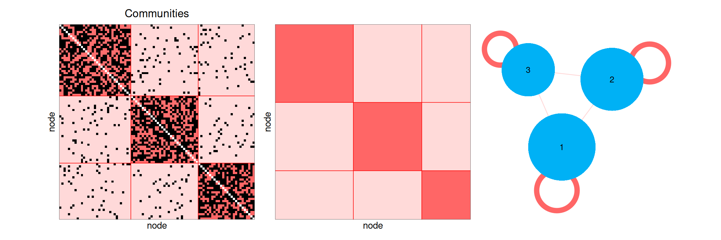

3.2 Core and periphery

A small block of nodes (the core) is connected to all the other nodes, whereas the nodes of the periphery are mostly connected to the core.

alphaCore <- matrix(c(0.9, 0.6, 0.3,
                      0.6, 0.2, 0.05,
                      0.3, 0.05, 0.01), 3, 3)
corePeriphery <- sampleSimpleSBM(nbNodes = 90, blockProp = c(0.15, 0.35, 0.5),
                                 connectParam = list(mean = alphaCore))
showSBM(corePeriphery, "Core and periphery")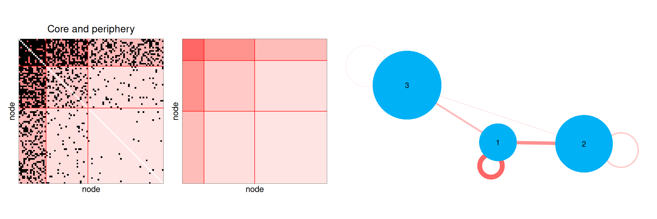

3.3 Disassortative structure

The nodes are connected to the nodes of the other block, not to the nodes of their own block, as in a network of sexual partners or a food web between predators and preys.

alphaDisassortative <- matrix(c(0.05, 0.6,
                                0.6, 0.05), 2, 2)
disassortative <- sampleSimpleSBM(nbNodes = 90, blockProp = c(0.5, 0.5),
                                  connectParam = list(mean = alphaDisassortative))
showSBM(disassortative, "Disassortative")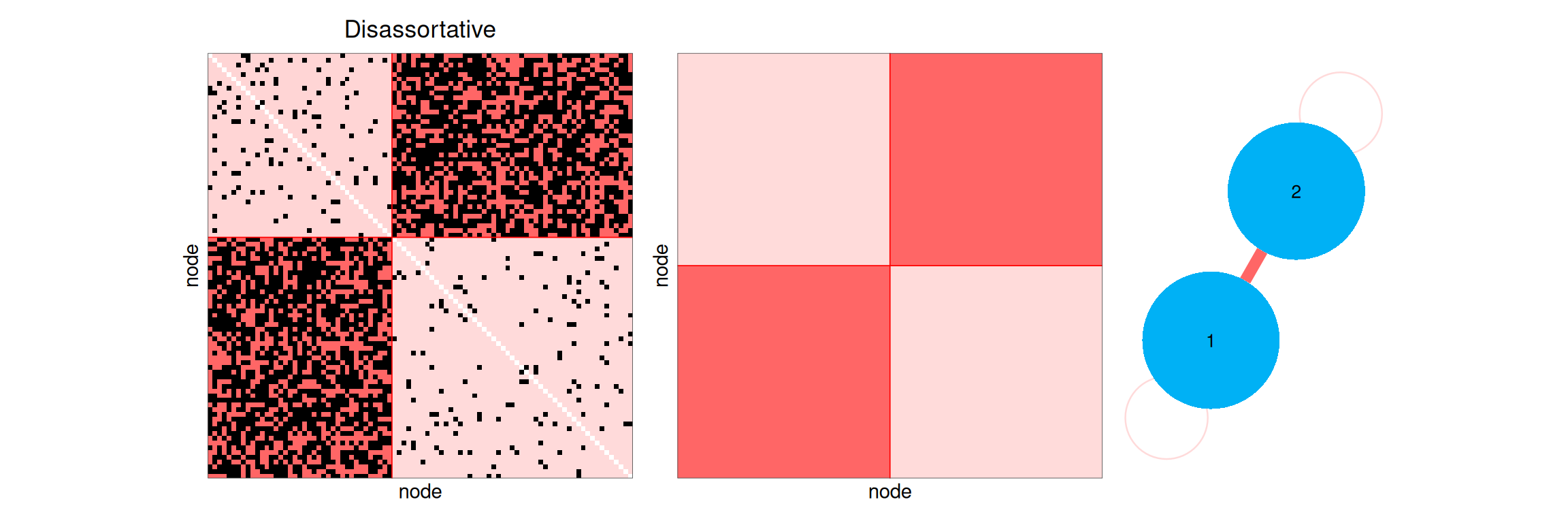

3.4 Hierarchy in a directed network

In a directed network, $\alpha_{ql}$ is the probability of an edge from a node of block $q$ to a node of block $l$, and the connectivity matrix is not symmetric. Here, the edges go mostly from block 1 to block 2 and from block 2 to block 3: the mesoscopic view displays the hierarchy with arrows.

alphaHierarchy <- matrix(c(0.2, 0.6, 0.3,
                           0.02, 0.2, 0.7,
                           0.01, 0.02, 0.2), 3, 3, byrow = TRUE)
hierarchy <- sampleSimpleSBM(nbNodes = 90, blockProp = c(0.3, 0.3, 0.4),
                             connectParam = list(mean = alphaHierarchy),
                             directed = TRUE)
showSBM(hierarchy, "Directed hierarchy")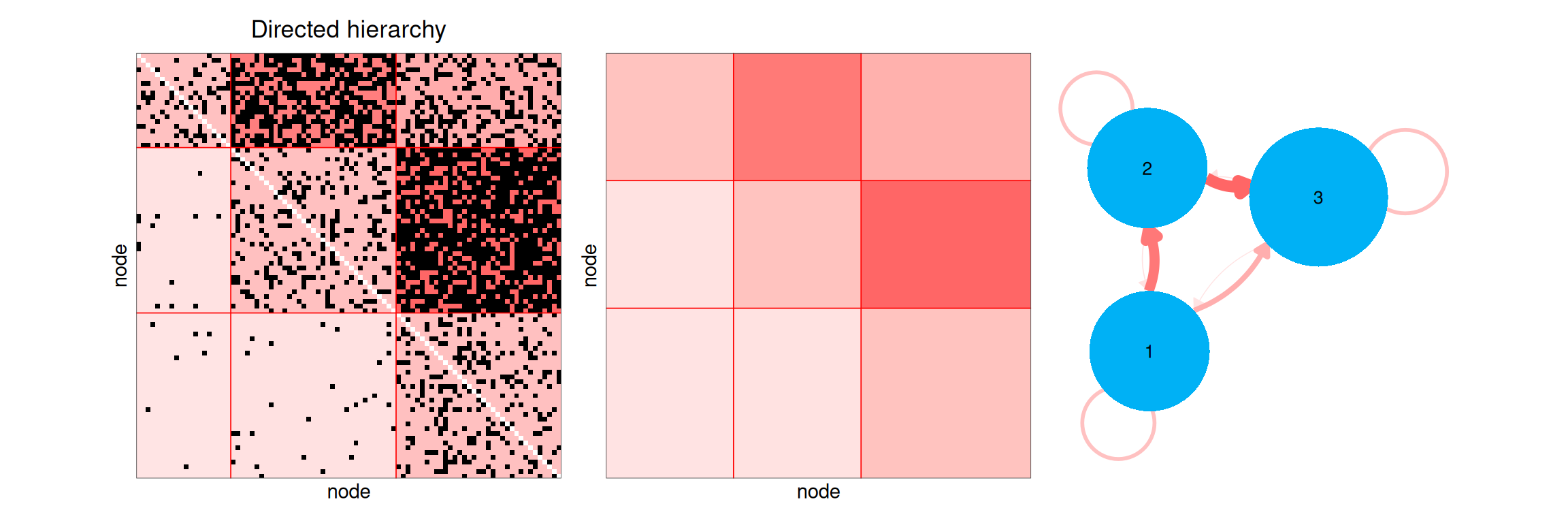

3.5 Count and weighted networks

With the Poisson distribution, $\alpha_{ql}$ is the mean number of interactions between a node of block $q$ and a node of block $l$; with the Gaussian distribution, it is the mean weight of the relation. The colors of the plots now represent the counts or the weights.

alphaPoisson <- matrix(c(8, 2, 0.5,
                         2, 4, 1,
                         0.5, 1, 0.2), 3, 3)
countNetwork <- sampleSimpleSBM(nbNodes = 90, blockProp = c(0.3, 0.3, 0.4),
                                connectParam = list(mean = alphaPoisson),
                                model = "poisson")
showSBM(countNetwork, "Poisson SBM")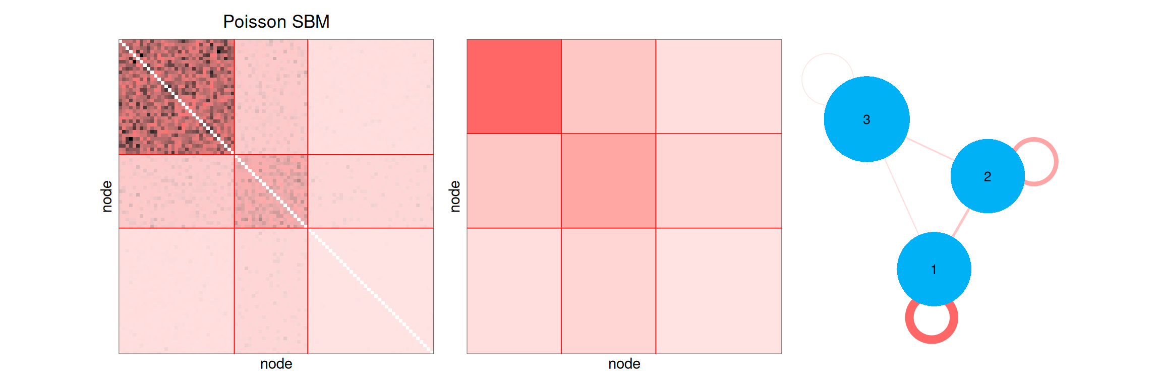

alphaGaussian <- matrix(c(4, 1, 0,
                          1, 3, 2,
                          0, 2, 1), 3, 3)
weightedNetwork <- sampleSimpleSBM(nbNodes = 90, blockProp = c(0.3, 0.3, 0.4),
                                   connectParam = list(mean = alphaGaussian, var = 1),
                                   model = "gaussian")
showSBM(weightedNetwork, "Gaussian SBM")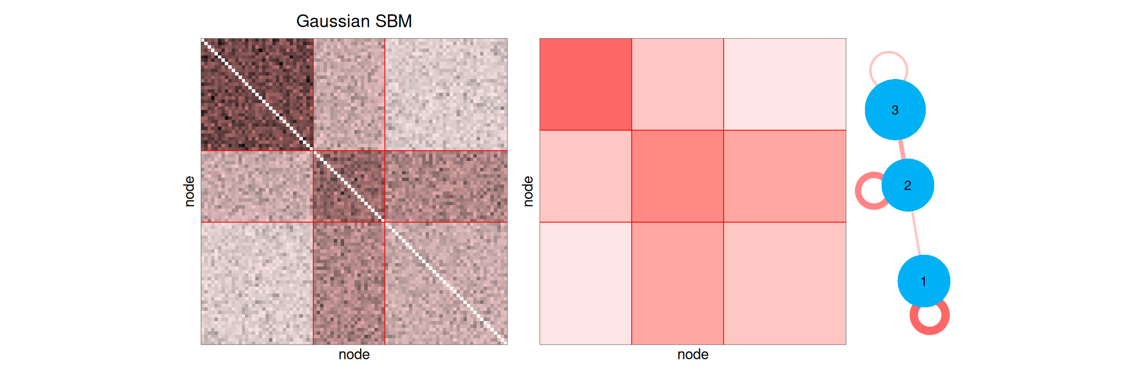

3.6 Bipartite networks

In a bipartite network, the mesoscopic view draws the blocks of rows (on top) and the blocks of columns (at the bottom) with different colors. A modular bipartite network is made of groups of rows interacting with their own group of columns.

alphaModular <- matrix(c(0.7, 0.05, 0.05,
                         0.05, 0.6, 0.05,
                         0.05, 0.05, 0.8), 3, 3)
modular <- sampleBipartiteSBM(nbNodes = c(60, 90),
                              blockProp = list(row = c(0.3, 0.4, 0.3), col = c(0.3, 0.3, 0.4)),
                              connectParam = list(mean = alphaModular),
                              dimLabels = c(row = "plant", col = "pollinator"))
showSBM(modular, "Modular bipartite network")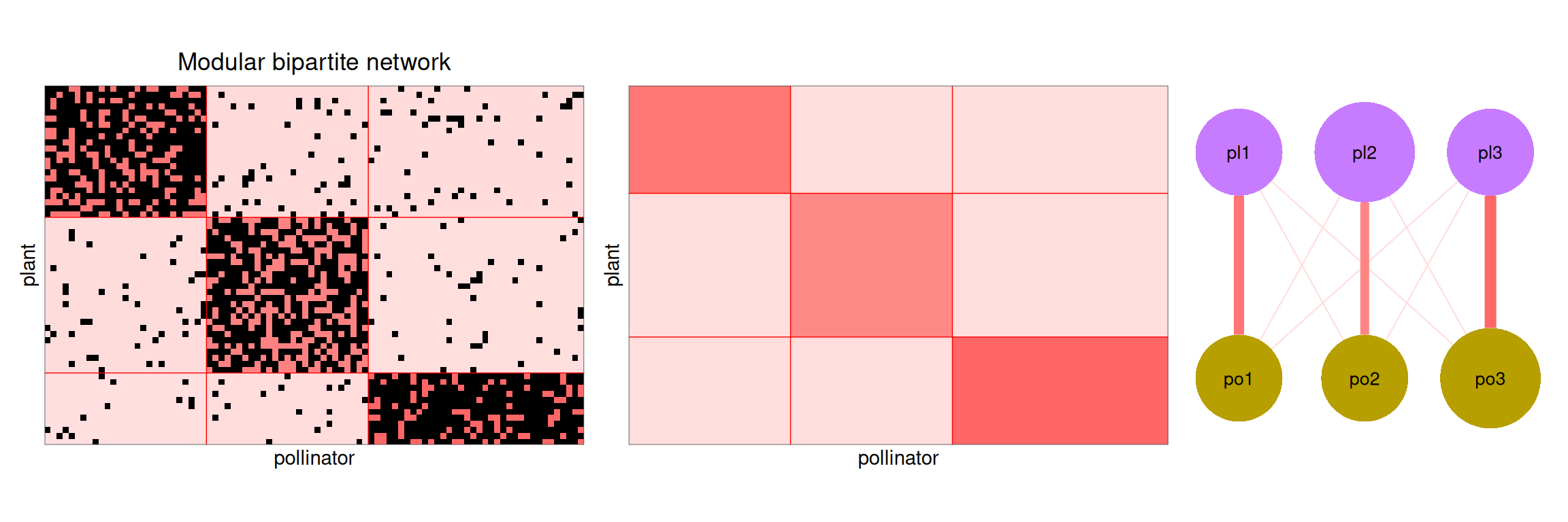

In a nested network, frequently observed in ecology, the specialists (rows or columns with few interactions) interact with a subset of the partners of the generalists.

alphaNested <- matrix(c(0.95, 0.8, 0.5,
                        0.8, 0.4, 0.1,
                        0.5, 0.1, 0.02), 3, 3)
nested <- sampleBipartiteSBM(nbNodes = c(60, 90),
                             blockProp = list(row = c(0.2, 0.3, 0.5), col = c(0.2, 0.3, 0.5)),
                             connectParam = list(mean = alphaNested),
                             dimLabels = c(row = "plant", col = "pollinator"))
showSBM(nested, "Nested bipartite network")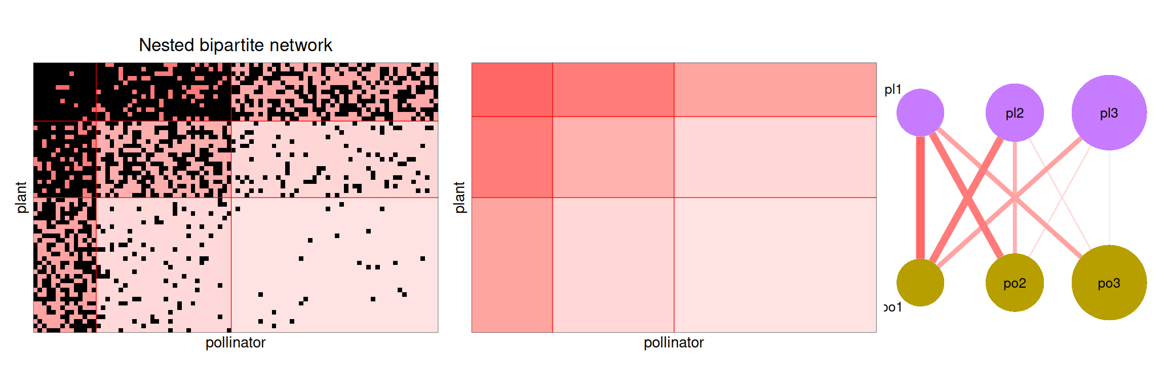

4. Inference

4.1 Estimation and model selection

The blocks and the parameters $\theta = (\pi, \alpha)$ are estimated with a variational EM algorithm (Leger 2016), which computes an approximation of the distribution of the blocks given the network, for each number of blocks $Q$ in a range explored by the algorithm. The number of blocks is selected with the Integrated Classification Likelihood (ICL). For a simple SBM with $Q$ blocks, the ICL computed by the package is $$\mathrm{ICL}(Q) = \mathbb{E}_{Z\sim p^{Var}}[\log \, p(Y, Z; \widehat{\theta})] - \frac{1}{2}\left[ N_\alpha \, \log \, N_{Y} + (Q-1)\, \log \, n \right],$$ where:

• $\mathbb{E}_{Z\sim p^{Var}}[\log p(Y, Z; \widehat{\theta})]$ is the complete-data log-likelihood, the latent blocks $Z$ being integrated against the variational distribution $p^{Var}$;
• $N_\alpha$ is the number of connectivity parameters: $Q^2$ for a directed network, $Q(Q+1)/2$ for an undirected one (plus one variance parameter in the Gaussian case). It is penalized by the logarithm of the number of dyads $N_Y$: $n(n-1)$ for a directed network, $n(n-1)/2$ for an undirected one;
• $Q-1$ is the number of free block proportions, penalized by the logarithm of the number of nodes $n$.

For a bipartite SBM, the penalty becomes $$N_\alpha \log(n_1 n_2) + (Q_1-1)\log n_1 + (Q_2-1)\log n_2,$$ with $N_\alpha = Q_1 Q_2$.

The model with the highest ICL is selected.

4.2 Fitting a simulated network

We fit an SBM on the core-periphery network simulated above with estimateSimpleSBM. The network being undirected and binary, we use a Bernoulli SBM.

fitCore <- estimateSimpleSBM(corePeriphery$networkData, model = "bernoulli",
                             estimOptions = list(verbosity = 0, plot = FALSE))

All the models explored during the estimation are stored in the field storedModels, which gives for each number of blocks the log-likelihood and the ICL.

fitCore$storedModels |>
  ggplot() + aes(x = nbBlocks, y = ICL) + geom_line() + geom_point() +
  geom_vline(xintercept = fitCore$nbBlocks, color = "red", linetype = "dashed")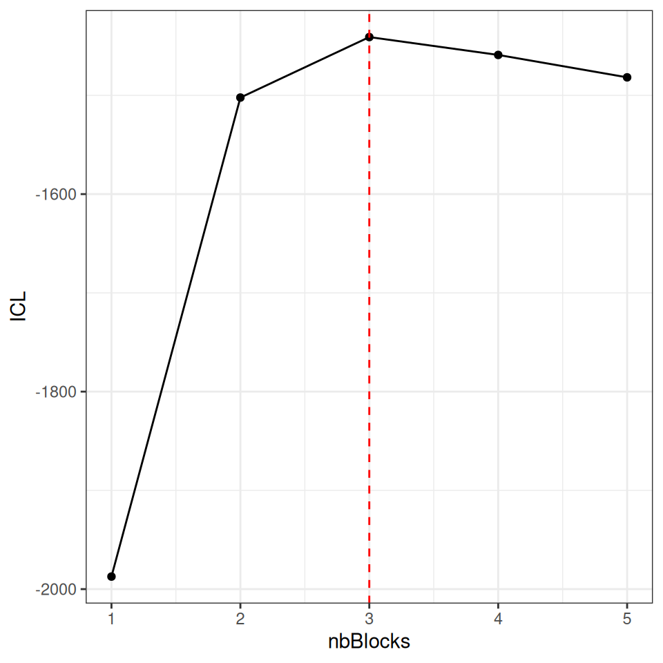

The ICL selects 3 blocks, the true number. The estimated blocks are compared with the true ones with a contingency table and the Adjusted Rand Index (ARI, equal to $1$ for a perfect recovery).

table(estimated = fitCore$memberships, true = corePeriphery$memberships)
#>          true
#> estimated  1  2  3
#>         1 17  0  0
#>         2  0 25  3
#>         3  0  1 44
aricode::ARI(fitCore$memberships, corePeriphery$memberships)
#> [1] 0.853803

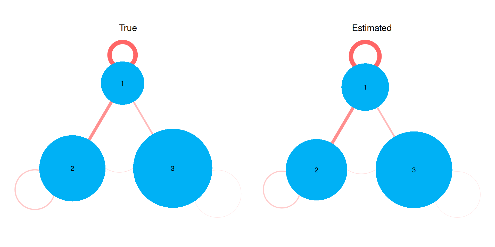
The estimated connectivity and block proportions are close to the true ones, up to a permutation of the blocks:

round(fitCore$connectParam$mean, 2)
#>      [,1] [,2] [,3]
#> [1,] 0.89 0.61 0.30
#> [2,] 0.61 0.18 0.05
#> [3,] 0.30 0.05 0.01
round(fitCore$blockProp, 2)
#> [1] 0.19 0.32 0.49

which can be seen by comparing the true and estimated mesoscopic views. To compare them, the blocks are placed at the same positions with the option layout (one row of coordinates per block); here, the estimated blocks have the same numbers as the true ones (see the table above), otherwise the rows of the layout should be permuted accordingly.

triangle <- cbind(x = c(0, -1, 1), y = c(1, -0.7, -0.7))
plot(corePeriphery, type = "meso", plotOptions = list(layout = triangle, title = "True")) |
  plot(fitCore, type = "meso", plotOptions = list(layout = triangle, title = "Estimated"))

5. The plots of the package

The plot method is available for the simulated networks and the fitted models, both for simple and bipartite SBM. Its argument type gives the representation:

type	Representation
"data"	the adjacency matrix, the nodes being ordered by block (option ordered = FALSE to keep the original order). The background of each block is colored according to its mean value
"expected"	the expected value of each edge under the model
"graphon"	the connectivity, each block being represented by an interval whose length is its proportion
"meso"	the mesoscopic view: the graphon drawn as a network

The expected value of each edge

We call expected value of each edge the value $$\mathbb{E}[Y_{ij}] = \sum_{q=1}^Q\sum_{r=1}^Q \widehat{\tau}^{var}_{iq}\widehat{\tau}^{var}_{jr} \widehat{\alpha}_{qr}$$ where $\widehat{\tau}^{var}_{iq} = \mathbb{P}(Z_i=q \mid y^{obs})$ approximated by the variational inference. This value is obtained by mySimpleSBM$predict().

All these plots are ggplot2 objects, which can be modified or combined (here with patchwork).

plot(fitCore, type = "data") | plot(fitCore, type = "expected")

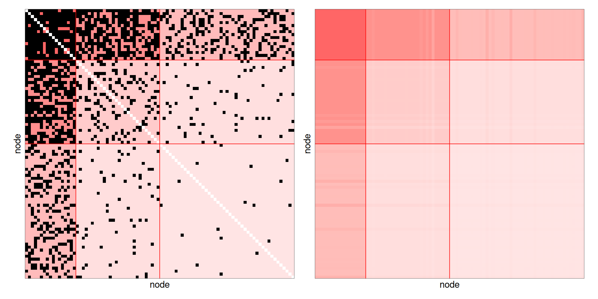
The plots are customized with the argument plotOptions (see ?plot.SBM for all the options). For instance, the names of the nodes are added to the matrix plots with rowNames = TRUE and colNames = TRUE. For the mesoscopic view:

• withinBlock = "fill" represents the connectivity within the blocks by the color of the blocks instead of loops (for simple SBM only, the colors of the blocks distinguishing the types of nodes in bipartite SBM);
• edge.threshold hides the connectivities below a threshold;
• seed fixes the random layout, which can also be given with layout;
• vertex.color, vertex.size, vertex.label.name change the colors, sizes and labels of the blocks.

plot(fitCore, type = "meso", plotOptions = list(seed = 1, withinBlock = "fill")) |
  plot(fitCore, type = "meso", plotOptions = list(seed = 1, edge.threshold = 0.1,
                                                  vertex.color = "steelblue"))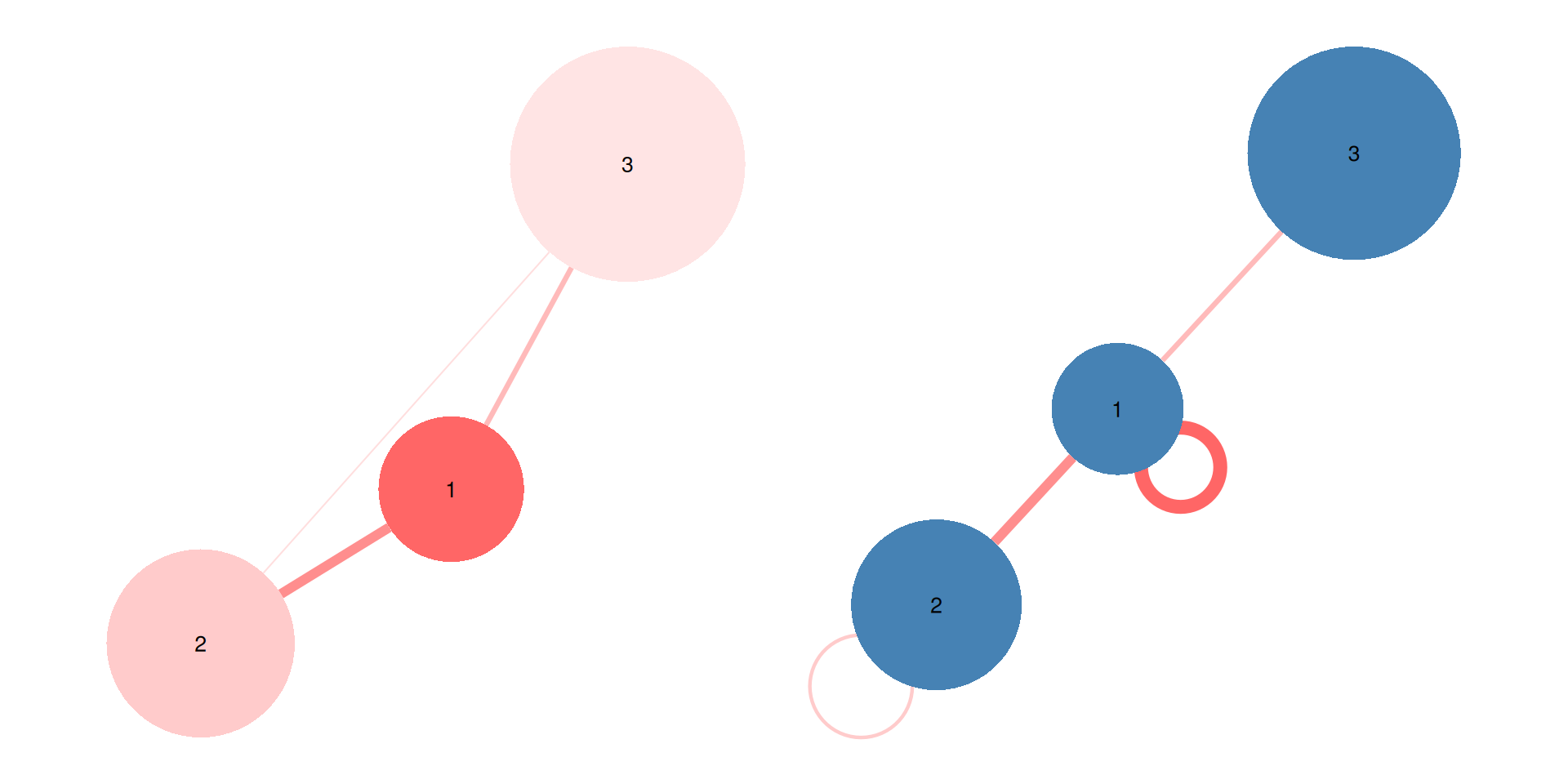

The matrix and the graphon of any network or connectivity can also be drawn directly with the functions plotMyMatrix and plotMyGraphon.

References

Leger, Jean-Benoist. 2016. “Blockmodels: A r-Package for Estimating in Latent Block Model and Stochastic Block Model, with Various Probability Functions, with or Without Covariates.” arXiv Preprint arXiv:1602.07587.