Stochastic Block Models for Multiplex networks
War and Alliance case study
team großBM
2024-09-16
Source:vignettes/Multiplex_allianceNwar_case_study.Rmd
Multiplex_allianceNwar_case_study.RmdPreliminaries
This vignette illustrates the use of the
estimateMultiplexSBM function and the methods accompanying
the R6 classes multiplexSBMfit on the war data
set.
Requirements
The packages required for the analysis are sbm plus some others for data manipulation and representation:
Data set
The war data set comes in the sbm
package:
data("war")This data set contains a list of two networks
(belligerent and alliance) where the nodes are
countries; an edge in the network belligerent means that
the two countries have been at war at least once between years 1816 to
2007; an edge in network alliance means that the two
countries have had a formal alliance between years 1816 and 2012. The
network belligerent have less nodes since countries which
have not been at war at all are not considered.
These two networks were extracted from https://correlatesofwar.org/ (see Sarkees and Wayman (2010) for war data, and Gibler (2008) for formal alliance). Version 4.0 was used for war data and version 4.1 for formal alliance.
Data manipulation
Since they don’t have the same size, we choose to only consider nodes (countries) which were at war with at least one other country. This corresponds to the first 83 nodes in the Alliance network.
A <- as.matrix(get.adjacency(war$alliance))
#> Warning: `get.adjacency()` was deprecated in igraph 2.0.0.
#> ℹ Please use `as_adjacency_matrix()` instead.
#> This warning is displayed once every 8 hours.
#> Call `lifecycle::last_lifecycle_warnings()` to see where this warning was
#> generated.
#> This graph was created by an old(er) igraph version.
#>   Call upgrade_graph() on it to use with the current igraph version
#>   For now we convert it on the fly...
A <- A[1:83, 1:83]
B <- as.matrix(get.adjacency(war$belligerent))
#> This graph was created by an old(er) igraph version.
#>   Call upgrade_graph() on it to use with the current igraph version
#>   For now we convert it on the fly...
We can start with a plot of this multiplex network:
netA <- defineSBM(A, model = "bernoulli", dimLabels = "country")
netB <- defineSBM(B, model = "bernoulli", dimLabels = "country")
plotMyMultiplexMatrix(list(netA, netB))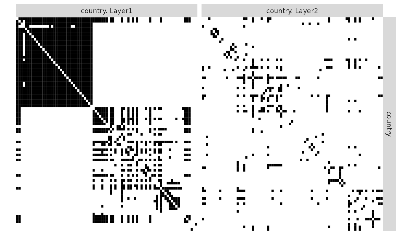
Fitting a multiplex SBM model where the two layers are assumed to be independent
We run the estimation of this multiplex model. By setting
dependent=FALSE, we declare that we consider the two layers
to be independent conditionally on the latent block variables.
MultiplexFitIndep <- estimateMultiplexSBM(list(netA, netB), dependent = FALSE,
    estimOptions = list(verbosity = 0))
We can retrieve the clustering
clust_country_indep <- MultiplexFitIndep$memberships[[1]]
sort(clust_country_indep)
#>       United States of America                         Canada
#>                              1                              1
#>                         Belize                    El Salvador
#>                              2                              2
#>                       Colombia                        Ecuador
#>                              2                              2
#>                        Bolivia                        Uruguay
#>                              2                              2
#>                        Bahamas                           Cuba
#>                              3                              3
#>                          Haiti             Dominican Republic
#>                              3                              3
#>                        Jamaica            Trinidad and Tobago
#>                              3                              3
#>                       Barbados                       Dominica
#>                              3                              3
#>                        Grenada                      St. Lucia
#>                              3                              3
#> St. Vincent and the Grenadines              Antigua & Barbuda
#>                              3                              3
#>            St. Kitts and Nevis                         Mexico
#>                              3                              3
#>                      Guatemala                       Honduras
#>                              3                              3
#>                      Nicaragua                     Costa Rica
#>                              3                              3
#>                         Panama                      Venezuela
#>                              3                              3
#>                         Guyana                       Suriname
#>                              3                              3
#>                           Peru                         Brazil
#>                              3                              3
#>                       Paraguay                          Chile
#>                              3                              3
#>                      Argentina                 United Kingdom
#>                              3                              4
#>                    Netherlands                        Belgium
#>                              4                              4
#>                     Luxembourg                         France
#>                              4                              4
#>                          Spain                       Portugal
#>                              4                              4
#>                        Germany        German Federal Republic
#>                              4                              4
#>                         Poland                        Hungary
#>                              4                              4
#>                 Czech Republic                          Italy
#>                              4                              4
#>                         Greece                         Norway
#>                              4                              4
#>                        Denmark                        Iceland
#>                              4                              4
#>                        Bavaria     German Democratic Republic
#>                              5                              5
#>                          Baden                   Wuerttemburg
#>                              5                              5
#>                Austria-Hungary                        Austria
#>                              5                              5
#>                 Czechoslovakia                       Slovakia
#>                              5                              5
#>                          Malta                        Albania
#>                              5                              5
#>                        Croatia                     Yugoslavia
#>                              5                              5
#>         Bosnia and Herzegovina                         Cyprus
#>                              5                              5
#>                       Bulgaria                        Moldova
#>                              5                              5
#>                        Romania                         Russia
#>                              5                              5
#>                        Estonia                         Latvia
#>                              5                              5
#>                      Lithuania                        Ukraine
#>                              5                              5
#>                        Belarus                        Armenia
#>                              5                              5
#>                        Georgia                     Azerbaijan
#>                              5                              5
#>                        Finland                         Sweden
#>                              5                              5
#>                     Cape Verde          Sao Tome and Principe
#>                              5                              5
#>                  Guinea-Bissau
#>                              5
And we can plot the reorganized adjacency matrices or the corresponding expectations:
plot(MultiplexFitIndep)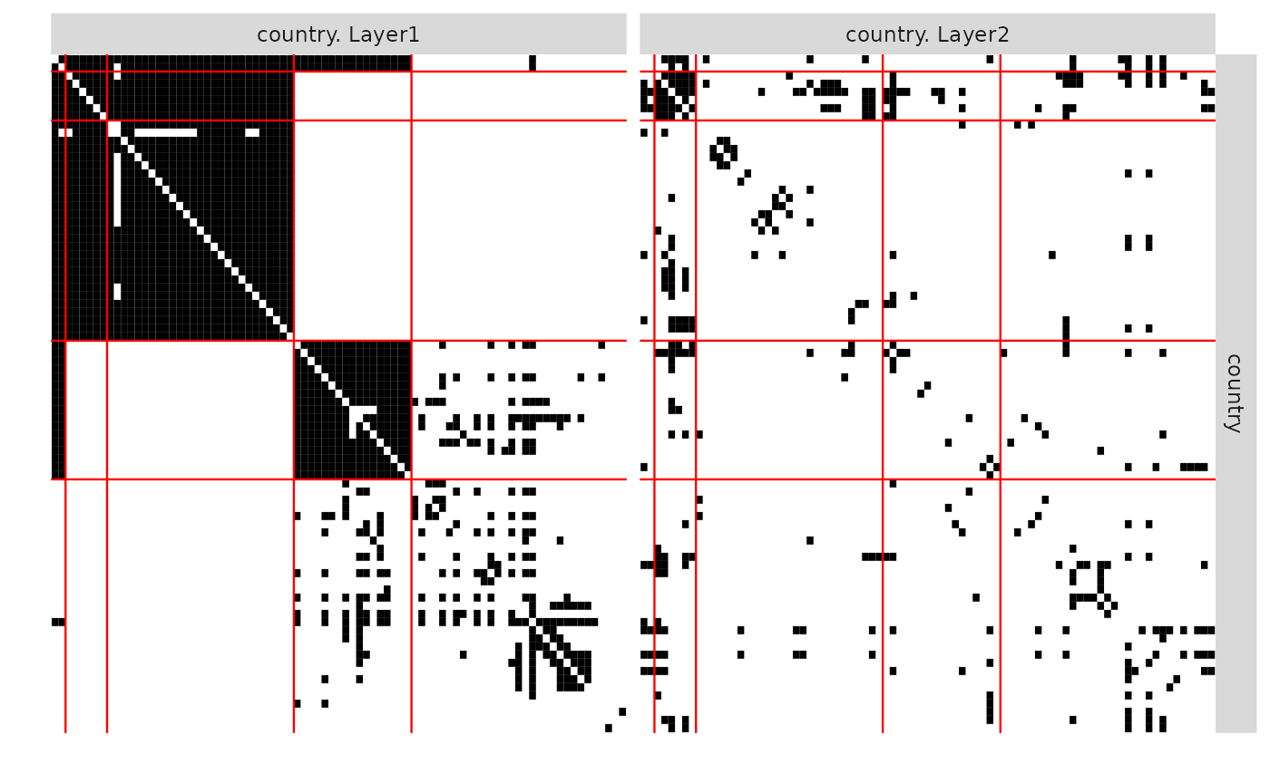
plot(MultiplexFitIndep, type = "expected")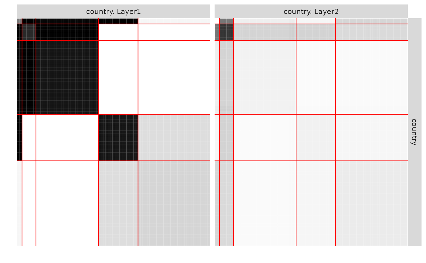
Fitting a multiplex SBM model where the two layers are assumed to be dependent
Now we assume that the two layers are dependent conditionally to the
latent block variables. We then set dependent = TRUE
MultiplexFitdep <- estimateMultiplexSBM(list(netA, netB), dependent = TRUE,
    estimOptions = list(verbosity = 0))
We can retrieve the clustering and compare it to the one obtained in the independent case.
clust_country_dep <- MultiplexFitdep$memberships[[1]]
sort(clust_country_indep)
#>       United States of America                         Canada
#>                              1                              1
#>                         Belize                    El Salvador
#>                              2                              2
#>                       Colombia                        Ecuador
#>                              2                              2
#>                        Bolivia                        Uruguay
#>                              2                              2
#>                        Bahamas                           Cuba
#>                              3                              3
#>                          Haiti             Dominican Republic
#>                              3                              3
#>                        Jamaica            Trinidad and Tobago
#>                              3                              3
#>                       Barbados                       Dominica
#>                              3                              3
#>                        Grenada                      St. Lucia
#>                              3                              3
#> St. Vincent and the Grenadines              Antigua & Barbuda
#>                              3                              3
#>            St. Kitts and Nevis                         Mexico
#>                              3                              3
#>                      Guatemala                       Honduras
#>                              3                              3
#>                      Nicaragua                     Costa Rica
#>                              3                              3
#>                         Panama                      Venezuela
#>                              3                              3
#>                         Guyana                       Suriname
#>                              3                              3
#>                           Peru                         Brazil
#>                              3                              3
#>                       Paraguay                          Chile
#>                              3                              3
#>                      Argentina                 United Kingdom
#>                              3                              4
#>                    Netherlands                        Belgium
#>                              4                              4
#>                     Luxembourg                         France
#>                              4                              4
#>                          Spain                       Portugal
#>                              4                              4
#>                        Germany        German Federal Republic
#>                              4                              4
#>                         Poland                        Hungary
#>                              4                              4
#>                 Czech Republic                          Italy
#>                              4                              4
#>                         Greece                         Norway
#>                              4                              4
#>                        Denmark                        Iceland
#>                              4                              4
#>                        Bavaria     German Democratic Republic
#>                              5                              5
#>                          Baden                   Wuerttemburg
#>                              5                              5
#>                Austria-Hungary                        Austria
#>                              5                              5
#>                 Czechoslovakia                       Slovakia
#>                              5                              5
#>                          Malta                        Albania
#>                              5                              5
#>                        Croatia                     Yugoslavia
#>                              5                              5
#>         Bosnia and Herzegovina                         Cyprus
#>                              5                              5
#>                       Bulgaria                        Moldova
#>                              5                              5
#>                        Romania                         Russia
#>                              5                              5
#>                        Estonia                         Latvia
#>                              5                              5
#>                      Lithuania                        Ukraine
#>                              5                              5
#>                        Belarus                        Armenia
#>                              5                              5
#>                        Georgia                     Azerbaijan
#>                              5                              5
#>                        Finland                         Sweden
#>                              5                              5
#>                     Cape Verde          Sao Tome and Principe
#>                              5                              5
#>                  Guinea-Bissau
#>                              5
aricode::ARI(clust_country_indep, clust_country_dep)
#> [1] 0.8886699
On top of the clustering comparison, we can compare the ICL criterion to see which of the dependent or independent models is a best fit:
MultiplexFitdep$ICL
#> [1] -1470.276
MultiplexFitIndep$ICL
#> [1] -1434.602
We can do the same plots for the reorganized matrices and the corresponding expectations. Note that the expectations correspond to the marginal expectation of each layer and it may be relevant to have a look at the conditional expectations.
plot(MultiplexFitdep)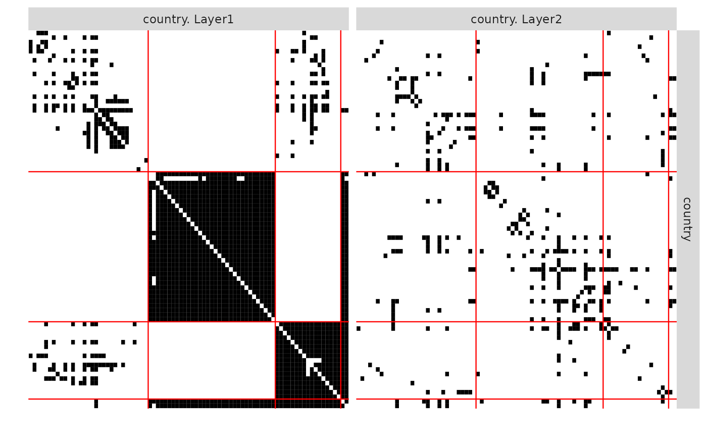
plot(MultiplexFitdep, type = "expected")
#> Warning in self$predict(): provided expectations are the marginal expectations
#> in the dependent case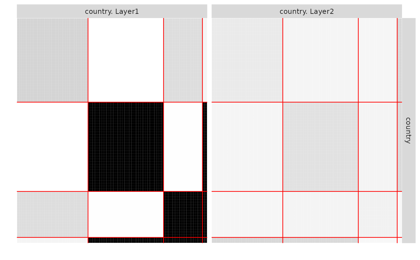
For instance, we may want to compare the marginal distribution for two countries in their given blocks to have being at war while they are allied at some point (before or after):
p11 <- MultiplexFitdep$connectParam$prob11
p01 <- MultiplexFitdep$connectParam$prob01
p10 <- MultiplexFitdep$connectParam$prob10
# conditional probabilities of being at war while having been or will
# be allied
round(p11/(p11 + p10), 2)
#>      [,1] [,2] [,3] [,4]
#> [1,] 0.09 0.10 0.03 0.43
#> [2,] 0.10 0.11 0.09 0.14
#> [3,] 0.03 0.09 0.05 0.03
#> [4,] 0.43 0.14 0.03 0.01
# marginal probabilities of being at war
round(p11 + p01, 2)
#>      [,1] [,2] [,3] [,4]
#> [1,] 0.07 0.04 0.03 0.14
#> [2,] 0.04 0.10 0.04 0.13
#> [3,] 0.03 0.04 0.05 0.03
#> [4,] 0.14 0.13 0.03 0.02