Multipartite Stochastic Block Models
An illustration on a mutualistic ecological network
team großBM
2024-09-16
Source:vignettes/Multipartite_EcologicalNetwork.Rmd
Multipartite_EcologicalNetwork.RmdPreliminaries
This vignette illustrates the use of the
estimateMultipartiteSBM function and the methods
accompanying the R6 classes `multipartiteSBMfit’.
Dataset
We apply our methodology to an ecological mutualistic multipartite
network.
The dataset –compiled and conducted by Dáttilo et
al. (2016) at Centro de
Investigaciones Costeras La Mancha (CICOLMA), located on the central
coast of the Gulf of Mexico, Veracruz, Mexico– involves three general
types of plant-animal mutualistic interaction: pollination, seed
dispersal by frugivorous birds, and protective mutualisms between ants
and plants with extrafloral nectaries.
The dataset –which is one of the largest compiled so far with respect to species richness, number of interactions and sampling effort– includes 4 functional groups (FG), namely plants, pollinator species (referred as floral visitors), ant species and frugivorous bird species. Three binary bipartite networks have been collected representing interactions between 1/ plants and florals visitor, 2/ plants and ants, and 3/ plants and seed dispersal birds, resulting into three bipartite networks.
The FG are of respective sizes: plant species, pollinator species, frugivorous bird species and ant species.
The 3 networks contain observed interactions of which are plant-pollinator interactions, are plant-birds interactions and are plant-ant interactions.
data(multipartiteEcologicalNetwork)
str(multipartiteEcologicalNetwork)
#> List of 3
#>  $ Inc_plant_ant   : int [1:141, 1:30] 0 1 0 0 1 0 1 0 1 0 ...
#>   ..- attr(*, "dimnames")=List of 2
#>   .. ..$ : chr [1:141] "Acacia_cornigera" "Acacia_macracantha" "Achatocarpus_nigricans" "Agave_angustifolia" ...
#>   .. ..$ : chr [1:30] "Camponotus_planatus" "Camponotus_mucronatus" "Paratrechina_longicornis_" "Crematogaster_brevispinosa" ...
#>  $ Inc_plant_bird  : int [1:141, 1:46] 0 0 1 0 0 0 0 0 0 0 ...
#>   ..- attr(*, "dimnames")=List of 2
#>   .. ..$ : chr [1:141] "Acacia_cornigera" "Acacia_macracantha" "Achatocarpus_nigricans" "Agave_angustifolia" ...
#>   .. ..$ : chr [1:46] "Cyanocorax_morio" "Tyrannus_forficatus" "Ortalis_vetula" "Myiozetetes_similis" ...
#>  $ Inc_plant_flovis: int [1:141, 1:173] 0 0 0 0 0 0 0 1 1 0 ...
#>   ..- attr(*, "dimnames")=List of 2
#>   .. ..$ : chr [1:141] "Acacia_cornigera" "Acacia_macracantha" "Achatocarpus_nigricans" "Agave_angustifolia" ...
#>   .. ..$ : chr [1:173] "Apis_melifera" "Lasioglossum_sp1" "Trigona_nigra" "Ascia_monuste" ...
names(multipartiteEcologicalNetwork)
#> [1] "Inc_plant_ant"    "Inc_plant_bird"   "Inc_plant_flovis"
Formatting the data
We format the data to be able to use our functions i.e. we transform
the matrices into an list containing the matrix, its
type : inc for incidence matrix, adj for
adjacency symmetric, and diradj for non symmetric
(oriented) adjacency matrix, the name of functional group in row and the
name of functional group in column. The three matrices are gathered in a
list.
To do so, we use the function defineNetwork.
Net <- multipartiteEcologicalNetwork
type = "bipartite"
model = "bernoulli"
directed = FALSE
PlantFlovis <- defineSBM(Net$Inc_plant_flovis, model, type, directed, dimLabels = c("Plants",
    "Flovis"))
PlantAnt <- defineSBM(Net$Inc_plant_ant, model, type, directed, dimLabels = c("Plants",
    "Ants"))
PlantBird <- defineSBM(Net$Inc_plant_bird, model, type, directed, dimLabels = c("Plants",
    "Birds"))
If one wants to keep a track of the names of the species, they should be used as rownames and colnames in the matrices.
PlantFlovis$netMatrix[1:2, 1:2]
#> NULL
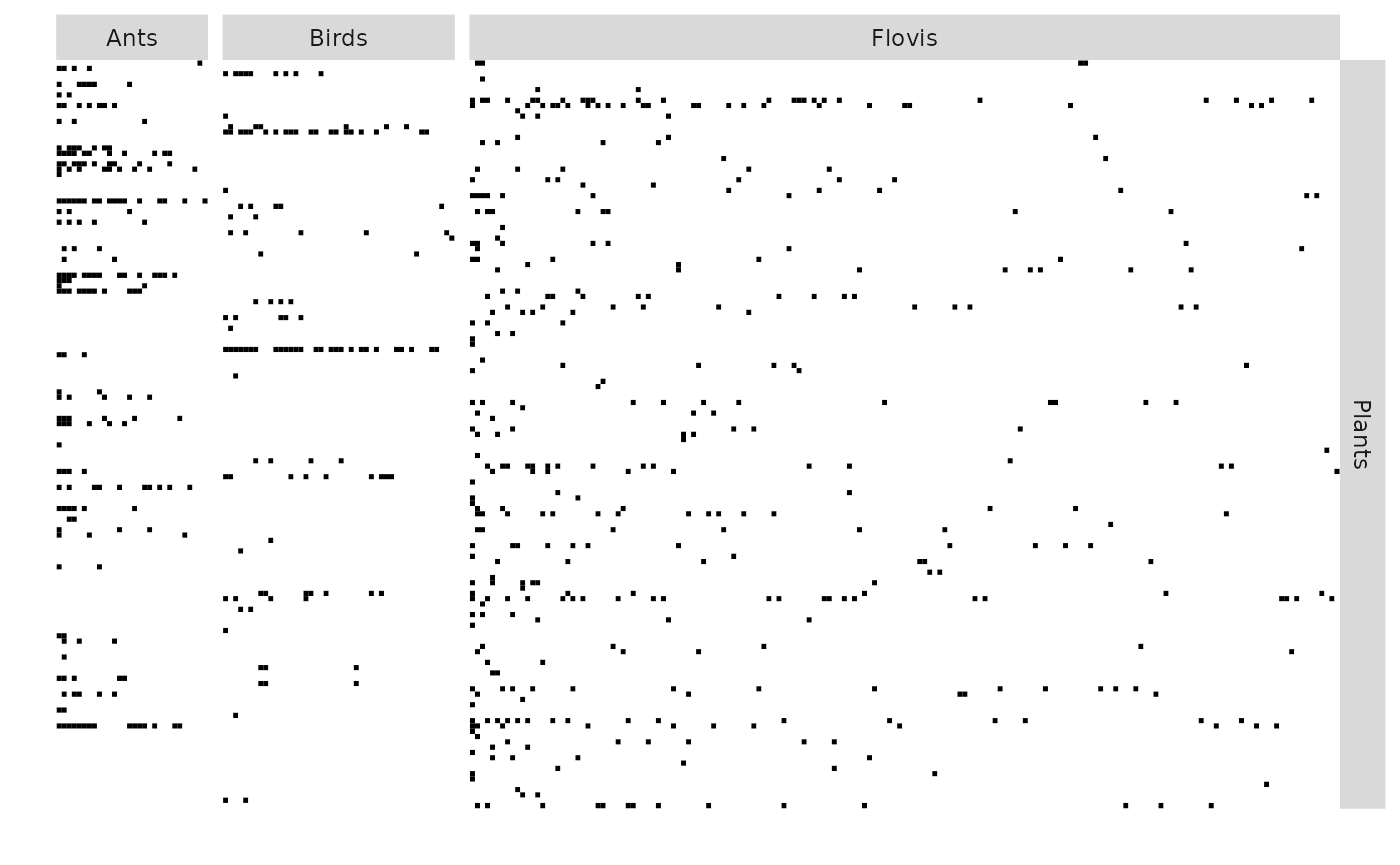
A plot of the data can be obtained with following command
plotMyMultipartiteMatrix(list(PlantFlovis, PlantAnt, PlantBird))
Mathematical Background
See Bar-Hen, Barbillon, and Donnet (2022) for details.
Inference
The model selection and the estimation are performed with the
function estimatemultipartiteBM.
estimOptions = list(initBM = FALSE)
listSBM <- list(PlantFlovis, PlantAnt, PlantBird)
myMSBM <- estimateMultipartiteSBM(listSBM, estimOptions)
contains the estimated parameters of the models we run through during the search of the better numbers of blocks.
myMSBM
#> Fit of a Multipartite Stochastic Block Model
#> 4 parts/functional groups ( Plants Flovis Ants Birds ),  3 networks
#> =====================================================================
#> nbNodes per FG = ( 141 173 30 46 ) --  nbBlocks per FG = ( 7 2 2 1 )
#> distributions on each network:  bernoulli bernoulli bernoulli
#> =====================================================================
#> * Useful fields
#>   $nbNetwork, $nbNodes, $nbBlocks, $dimLabels, $architecture
#>   $modelName, $blockProp, $connectParam, $memberships, $networkData
#>   $probMemberships, $loglik, $ICL, $storedModels,
#> * R6 and S3 methods
#>   plot, print, coef, predict, fitted, $setModel, $reorder
The best model has the following numbers of blocks:
myMSBM$nbBlocks
#> Plants Flovis   Ants  Birds
#>      7      2      2      1
To see the parameters estimated for the better model we use the
following command myMSBM$connectParam or
myMSBM$blockProp:
myMSBM$blockProp
#> $Plants
#> [1] 0.01418720 0.03802305 0.07840873 0.16063183 0.10614897 0.13507513 0.46752510
#>
#> $Flovis
#> [1] 0.06221568 0.93778432
#>
#> $Ants
#> [1] 0.1014381 0.8985619
#>
#> $Birds
#> [1] 1
myMSBM$connectParam
#> [[1]]
#> [[1]]$mean
#>              [,1]         [,2]
#> [1,] 2.464664e-15 4.440892e-16
#> [2,] 1.001131e-15 4.440892e-16
#> [3,] 1.651832e-01 3.427940e-02
#> [4,] 4.173707e-03 8.566580e-08
#> [5,] 1.917898e-01 6.378749e-02
#> [6,] 8.826487e-07 3.317267e-04
#> [7,] 9.573240e-02 7.490241e-03
#>
#>
#> [[2]]
#> [[2]]$mean
#>              [,1]         [,2]
#> [1,] 5.366301e-15 1.107167e-15
#> [2,] 8.491907e-01 3.564830e-01
#> [3,] 6.620266e-01 1.542027e-01
#> [4,] 5.430946e-01 5.891885e-02
#> [5,] 7.172257e-16 4.440892e-16
#> [6,] 5.721732e-16 4.440892e-16
#> [7,] 4.440892e-16 5.576222e-04
#>
#>
#> [[3]]
#> [[3]]$mean
#>              [,1]
#> [1,] 5.108074e-01
#> [2,] 4.440892e-16
#> [3,] 4.440892e-16
#> [4,] 4.440892e-16
#> [5,] 1.625224e-02
#> [6,] 7.534085e-02
#> [7,] 1.253527e-03
The clustering supplied by the better model are in
myMSBM$memberships$***.
table(myMSBM$memberships$Plants)
#>
#>  1  2  3  4  5  6  7
#>  2  5 11 23 15 20 65
table(myMSBM$memberships$Ants)
#>
#>  1  2
#>  3 27
myMSBM$storedModels
#>   indexModel nbParams nbBlocks Plants nbBlocks Flovis nbBlocks Ants
#> 1          1       43               7               2             2
#> 2          2       37               6               2             2
#> 3          3       31               5               2             2
#> 4          4       25               5               2             1
#> 5          5       19               5               1             1
#> 6          6       15               4               1             1
#> 7          7       11               3               1             1
#> 8          8        7               2               1             1
#> 9          9        3               1               1             1
#>   nbBlocks Birds nbBlocks       ICL    loglik
#> 1              1       12 -2961.903 -2770.230
#> 2              1       11 -2965.539 -2800.546
#> 3              1       10 -2981.164 -2840.532
#> 4              1        9 -3017.651 -2897.765
#> 5              1        8 -3071.369 -2984.442
#> 6              1        7 -3128.286 -3057.690
#> 7              1        6 -3216.136 -3161.801
#> 8              1        5 -3358.851 -3326.480
#> 9              1        4 -3582.348 -3568.733
Plots
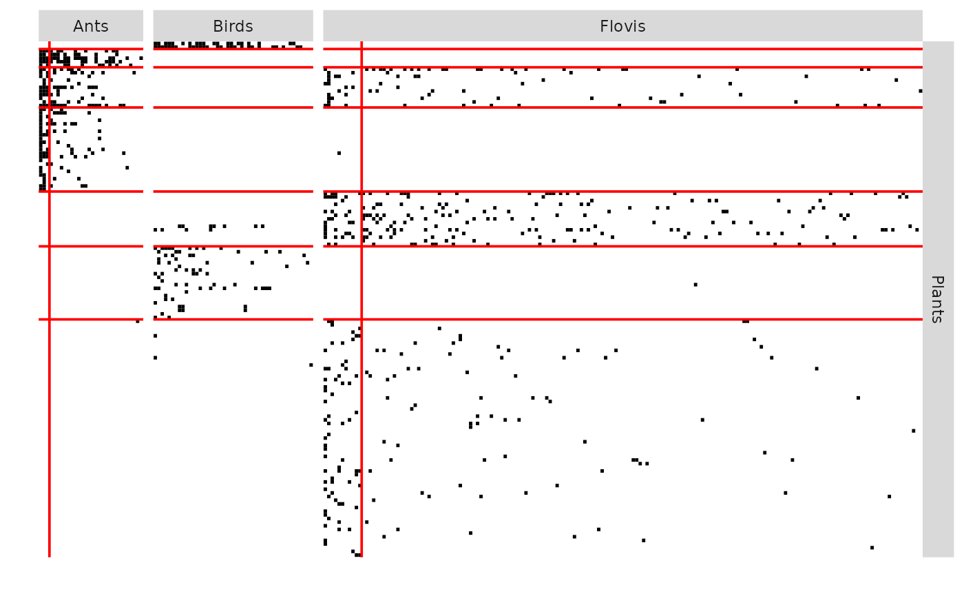
We can either plot the reorganized matrix:
plot(myMSBM) 
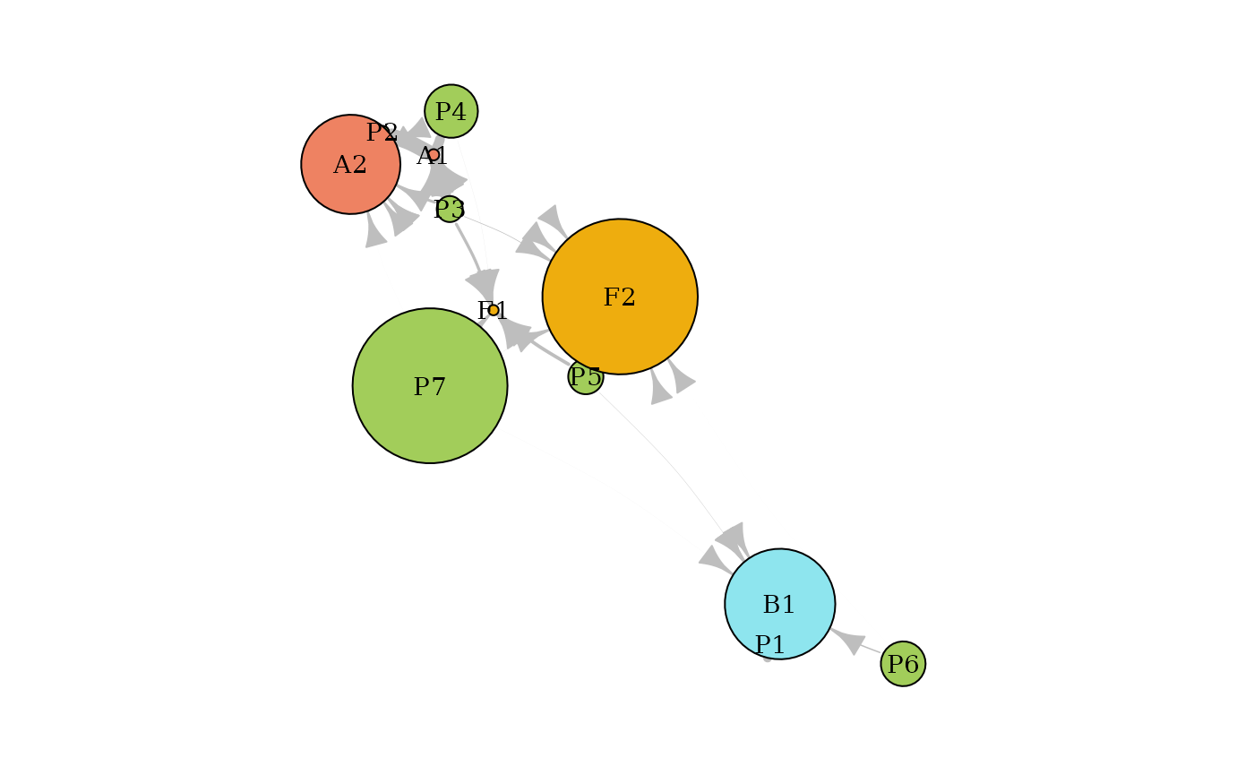
or the mesoscopic view:
plotOptions = list(vertex.size = c(12, 6, 4, 4))
plotOptions$vertex.shape = rep("circle", 4)
plotOptions$vertex.color = c("darkolivegreen3", "darkgoldenrod2", "salmon2",
    "cadetblue2")
plotOptions$edge.curved = 0.1
plot(myMSBM, type = "meso", plotOptions = plotOptions)