Simple and Bipartite Stochastic Block Models

Preliminaries

This vignette illustrates the use of the estimateSBM function and the methods accompanying the R6 classes SimpleSBMfit and BipartiteSBMfit.

Requirements

The packages required for the analysis are sbm plus some others for data manipulation and representation:

library(sbm)
library(ggplot2)
library(knitr)
theme_set(theme_bw())

Data set: antagonistic tree/fungus interaction network

We consider the fungus-tree interaction network studied by Vacher, Piou, and Desprez-Loustau (2008), available with the package sbm:

data("fungusTreeNetwork")
str(fungusTreeNetwork, max.level = 1)
#> List of 5
#>  $ tree_names  : Factor w/ 51 levels "Abies alba","Abies grandis",..: 1 2 3 14 42 4 5 6 7 8 ...
#>  $ fungus_names: Factor w/ 154 levels "Amphiporthe leiphaemia",..: 1 2 3 4 5 6 7 8 9 10 ...
#>  $ tree_tree   : num [1:51, 1:51] 0 12 9 3 2 2 0 0 2 7 ...
#>  $ fungus_tree : int [1:154, 1:51] 0 0 0 0 1 1 1 0 0 0 ...
#>  $ covar_tree  :List of 3

This data set provides information about $154$ fungi sampled on $51$ tree species. It is a list with the following entries:

fungi_list: list of the fungus species names
tree_list : list of the tree species names
fungus_tree : binary fungus-tree interactions
tree_tree : weighted tree-tree interactions (number of common fungal species two tree species host)
covar_tree : covariates associated to pairs of trees (namely genetic, taxonomic and geographic distances)

We first consider the tree-tree interactions resulting into a Simple Network. Then we consider the bipartite network between trees and fungi.

Mathematical Background

See Leger (2016) for details.

Analysis of the tree/tree data

Tree-tree binary interaction networks

We first consider the binary network where an edge is drawn between two trees when they do share a least one common fungi:

tree_tree_binary <- 1 * (fungusTreeNetwork$tree_tree != 0)

The simple function plotMyMatrix can be use to represent simple or bipartite SBM:

plotMyMatrix(tree_tree_binary, dimLabels =c('tree'))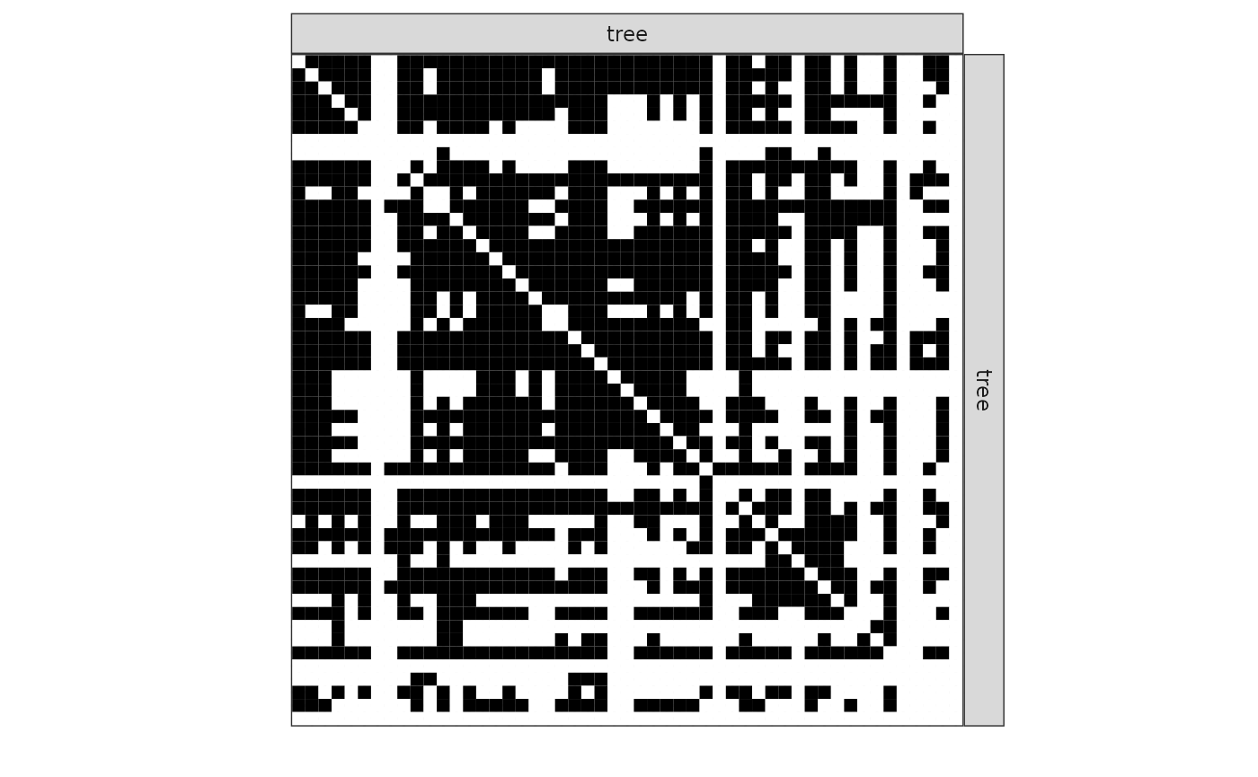

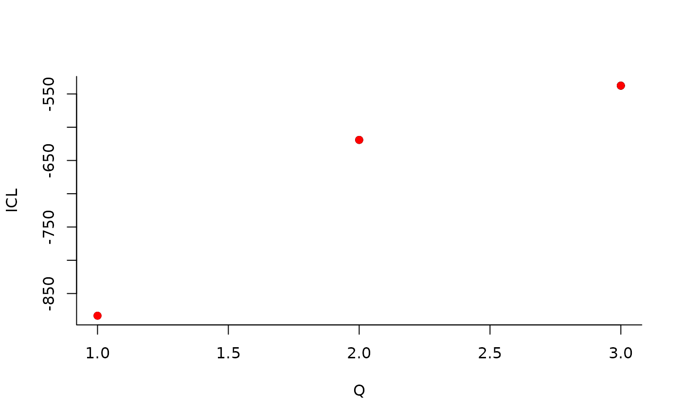
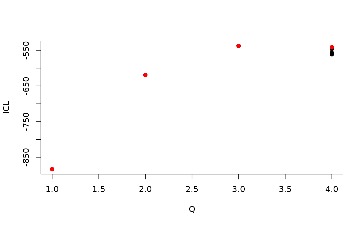
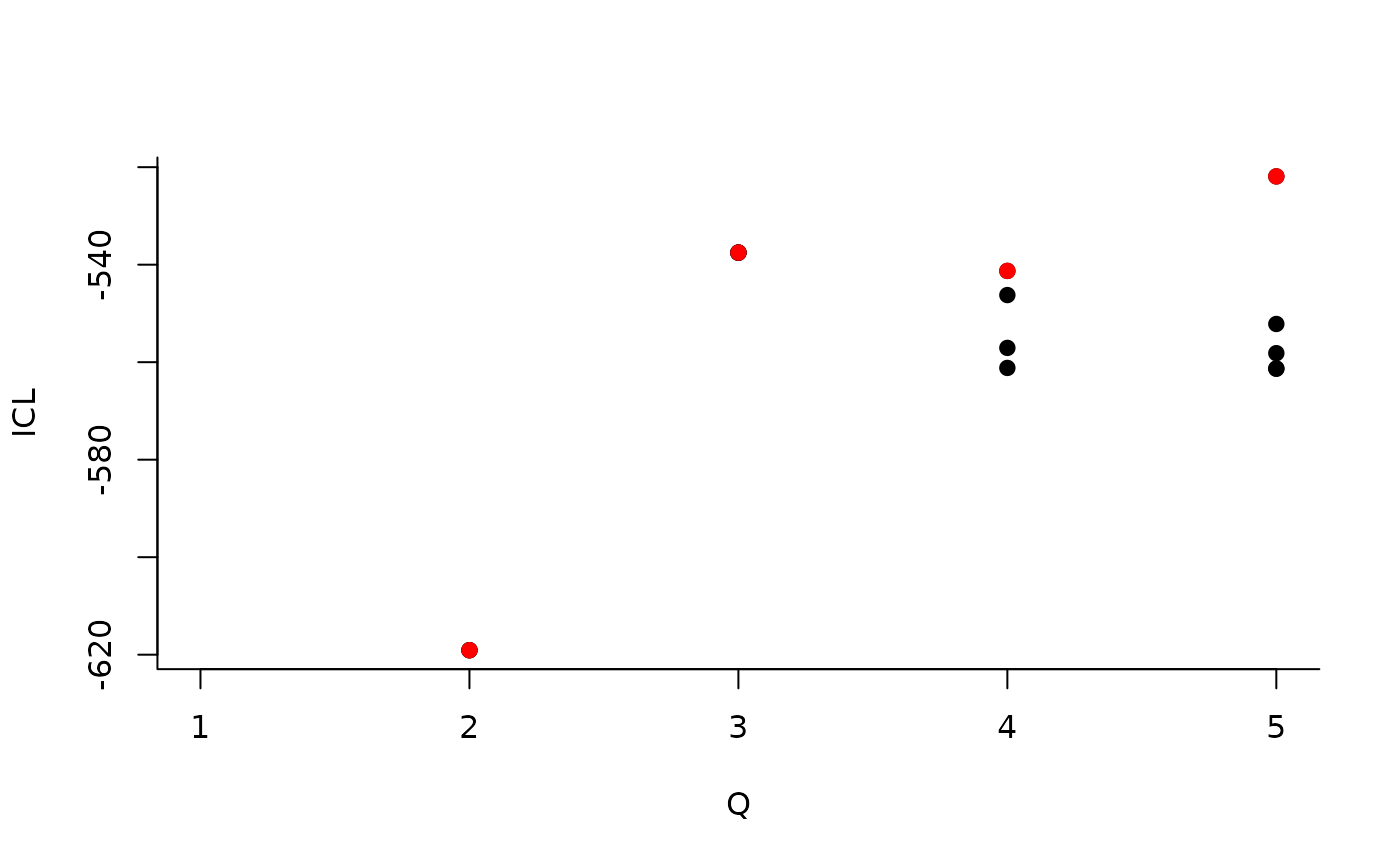
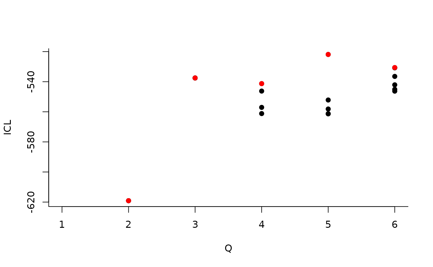
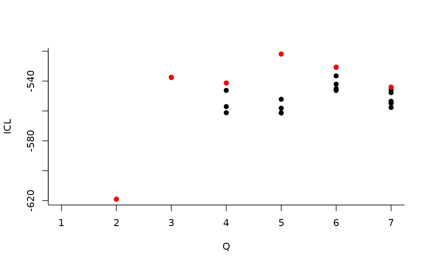
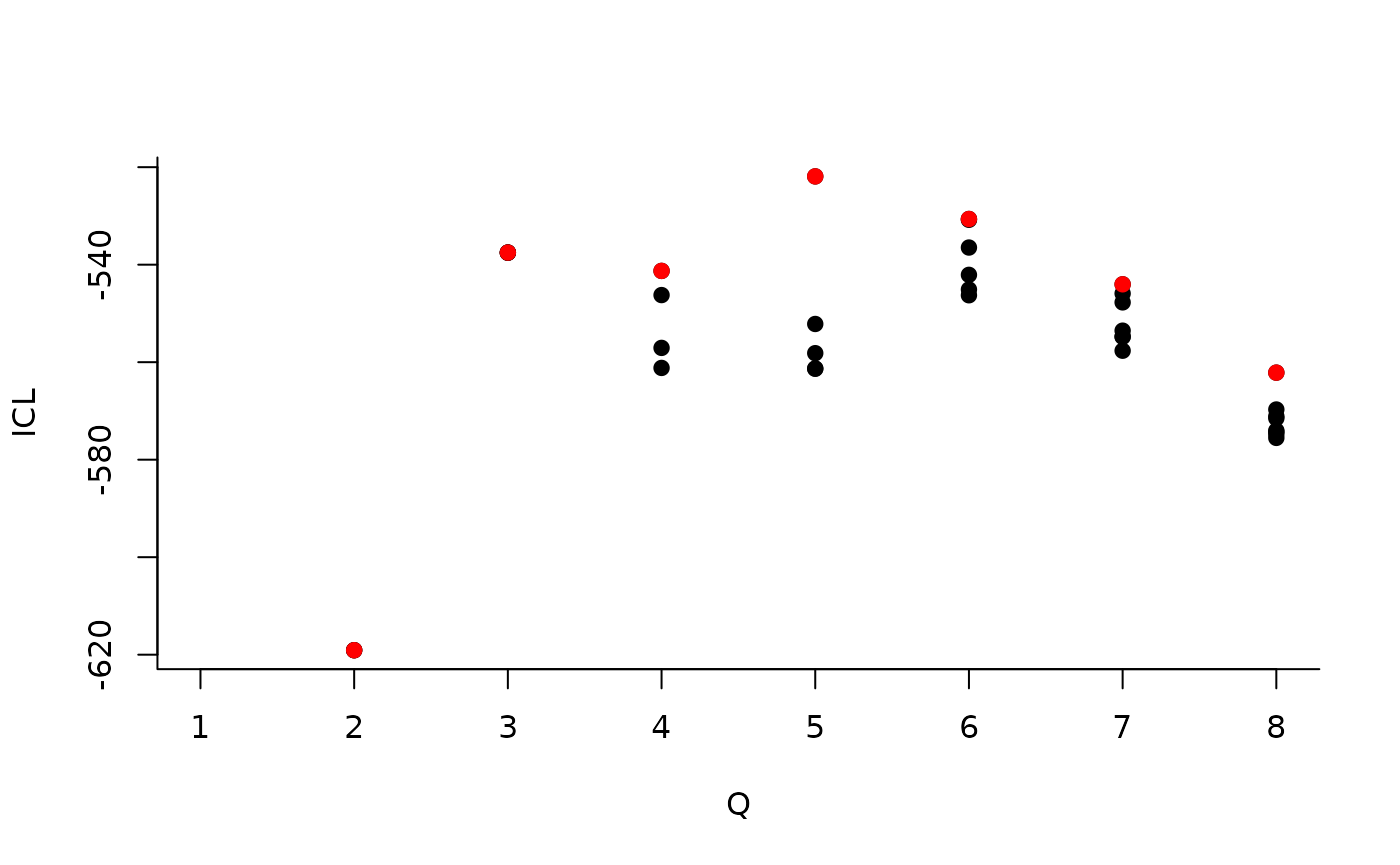
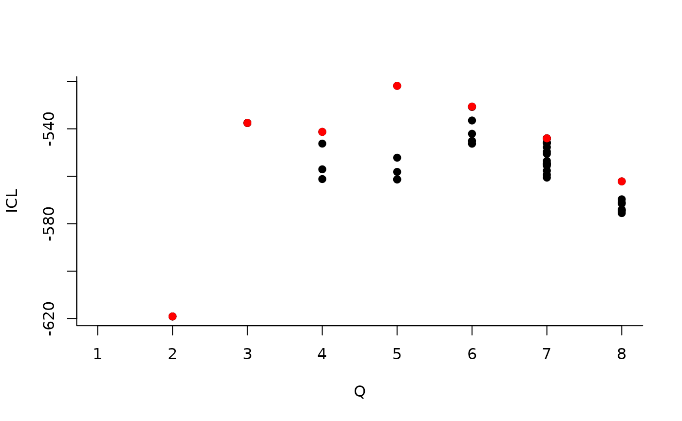
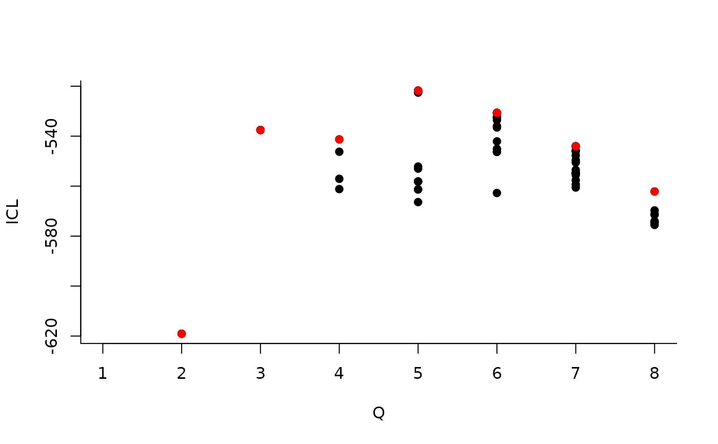
We look for some latent structure of the network by adjusting a simple SBM with the function estimateSimpleSBM.

mySimpleSBM <- tree_tree_binary %>% 
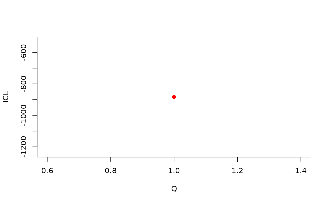
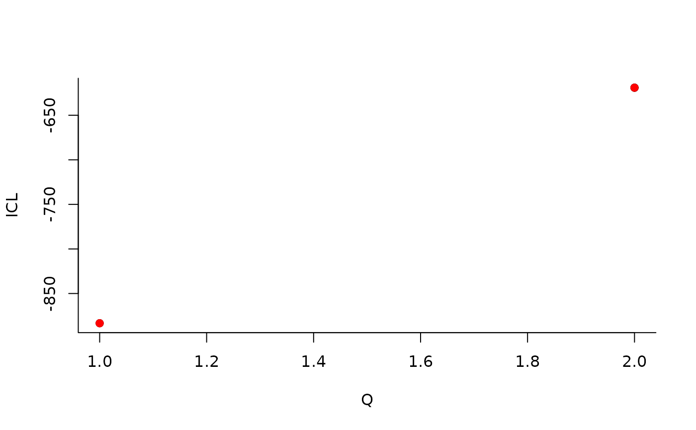
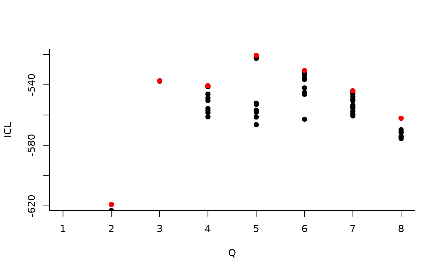
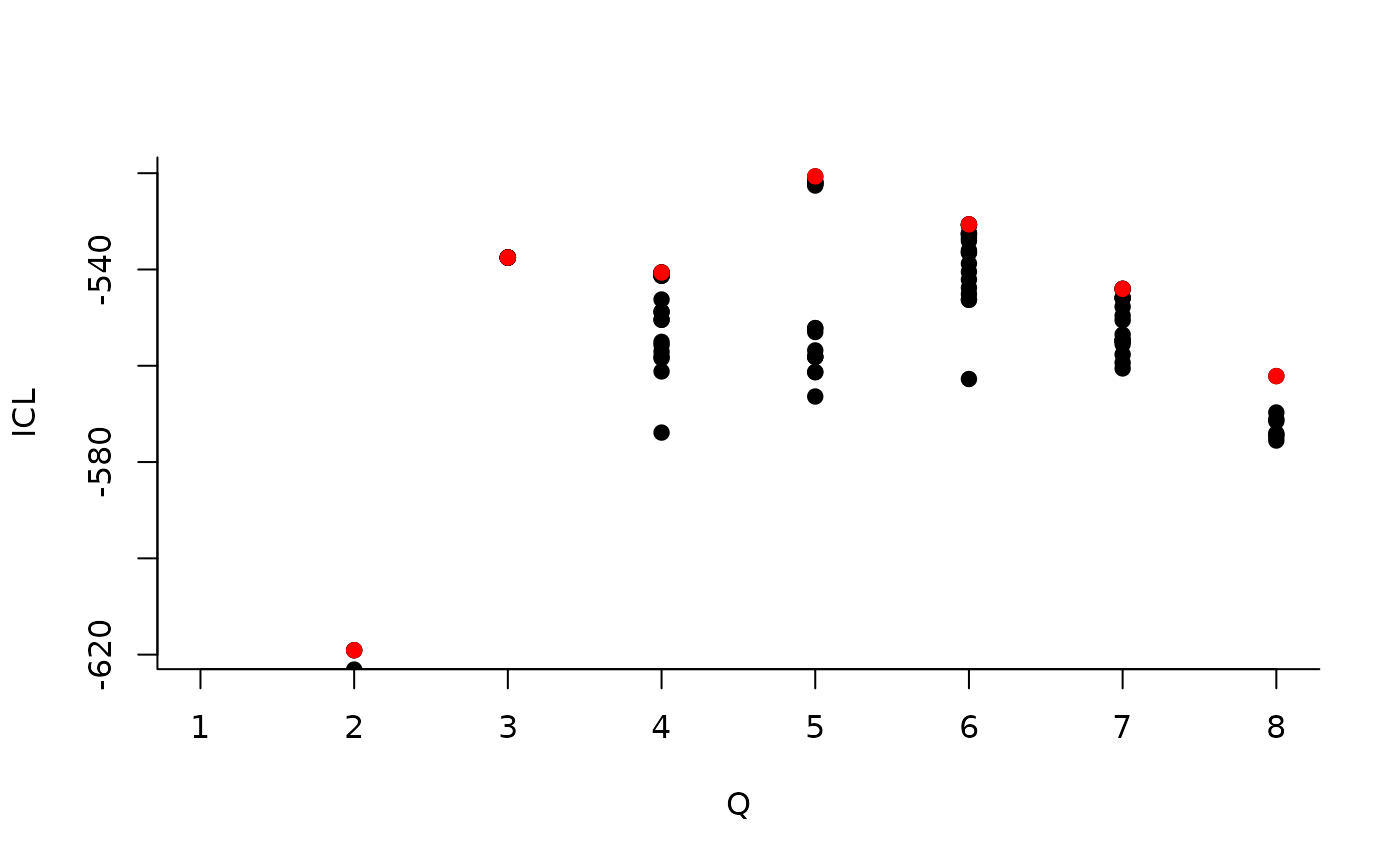
  estimateSimpleSBM("bernoulli", dimLabels = 'tree', estimOptions = list(verbosity = 1, plot = TRUE))
#> -> Estimation for 1 groups
#>

#> -> Computation of eigen decomposition used for initalizations
#> 
#> -> Pass 1
#>

#> -> Pass 2
#>

#> -> Pass 3

Once fitted, the user can manipulate the fitted model by accessing the various fields and methods enjoyed by the class simpleSBMfit. Most important fields and methods are recalled to the user via the show method:

class(mySimpleSBM)
#> [1] "SimpleSBM_fit" "SimpleSBM"     "SBM"           "R6"
mySimpleSBM
#> Fit of a Simple Stochastic Block Model -- bernoulli variant
#> =====================================================================
#> Dimension = ( 51 ) - ( 5 ) blocks and no covariate(s).
#> =====================================================================
#> * Useful fields 
#>   $nbNodes, $modelName, $dimLabels, $nbBlocks, $nbCovariates, $nbDyads
#>   $blockProp, $connectParam, $covarParam, $covarList, $covarEffect 
#>   $expectation, $indMemberships, $memberships 
#> * R6 and S3 methods 
#>   $rNetwork, $rMemberships, $rEdges, plot, print, coef 
#> * Additional fields
#>   $probMemberships, $loglik, $ICL, $storedModels, 
#> * Additional methods 
#>   predict, fitted, $setModel, $reorder

For instance,

mySimpleSBM$nbBlocks
#> [1] 5
mySimpleSBM$nbNodes
#> tree 
#>   51
mySimpleSBM$nbCovariates
#> [1] 0

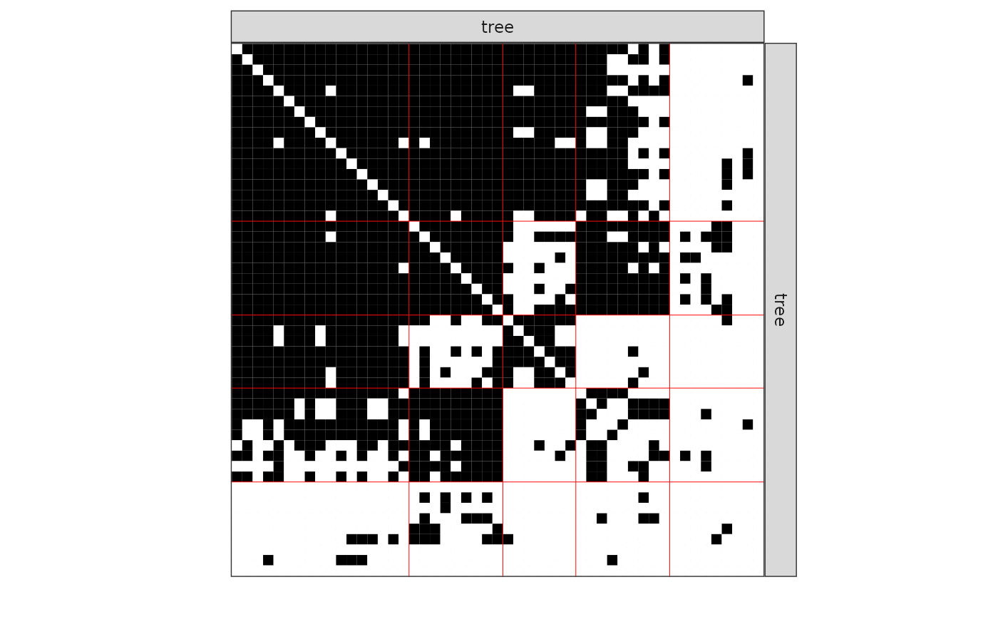
The plot method is available as a S3 or R6 method. The default represents the network data reordered according to the memberships estimated in the SBM.

plot(mySimpleSBM, type = "data", dimLabels  = c('tree'))

One can also plot the expected network which, in case of the Bernoulli model, corresponds to the probability of connection between any pair of nodes in the network.

plot(mySimpleSBM, type = "expected")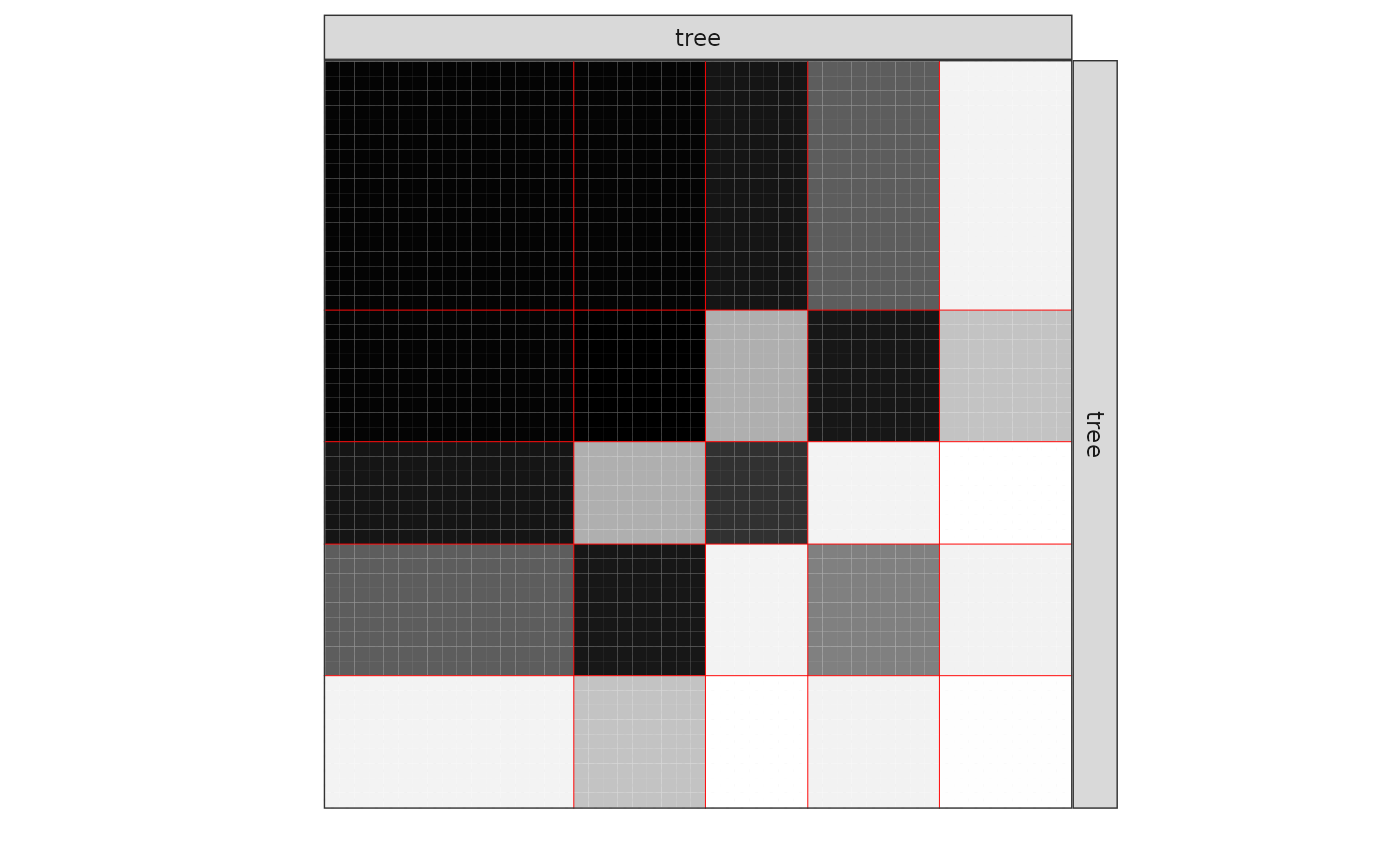

plot(mySimpleSBM, type = "meso")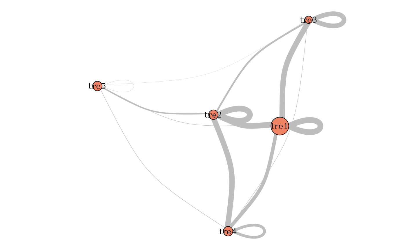

coef(mySimpleSBM, 'block')
#> [1] 0.3320954 0.1766383 0.1378665 0.1766999 0.1766999
coef(mySimpleSBM, 'connectivity')
#> $mean
#>            [,1]      [,2]       [,3]       [,4]       [,5]
#> [1,] 0.98230909 0.9828930 0.92749023 0.60851311 0.05994511
#> [2,] 0.98289303 0.9937459 0.29390960 0.91904879 0.22617761
#> [3,] 0.92749023 0.2939096 0.79890626 0.05802394 0.02169247
#> [4,] 0.60851311 0.9190488 0.05802394 0.47209785 0.06626655
#> [5,] 0.05994511 0.2261776 0.02169247 0.06626655 0.02899357

About model selection and choice of the number of blocks

During the estimation, a certain range of models are explored corresponding to different number of blocks. By default, the best model in terms of Integrated Classification Likelihood is sent back. In fact, all the model are stored internally. The user can have a quick glance at them via the $storedModels field:

mySimpleSBM$storedModels %>% kable()

indexModel	nbParams	nbBlocks	ICL	loglik
1	1	1	-883.3334	-879.7581
2	4	2	-619.0799	-606.3880
3	8	3	-537.5179	-512.1339
4	13	4	-540.6318	-498.9806
5	19	5	-520.6645	-459.1706
6	26	6	-530.6278	-445.7159
7	34	7	-544.0191	-432.1138
8	43	8	-562.1450	-419.6710

We can then see what models are competitive in terms of model selection by checking the ICL:

mySimpleSBM$storedModels %>%  ggplot() + aes(x = nbBlocks, y = ICL)  + geom_line() + geom_point(alpha = 0.5)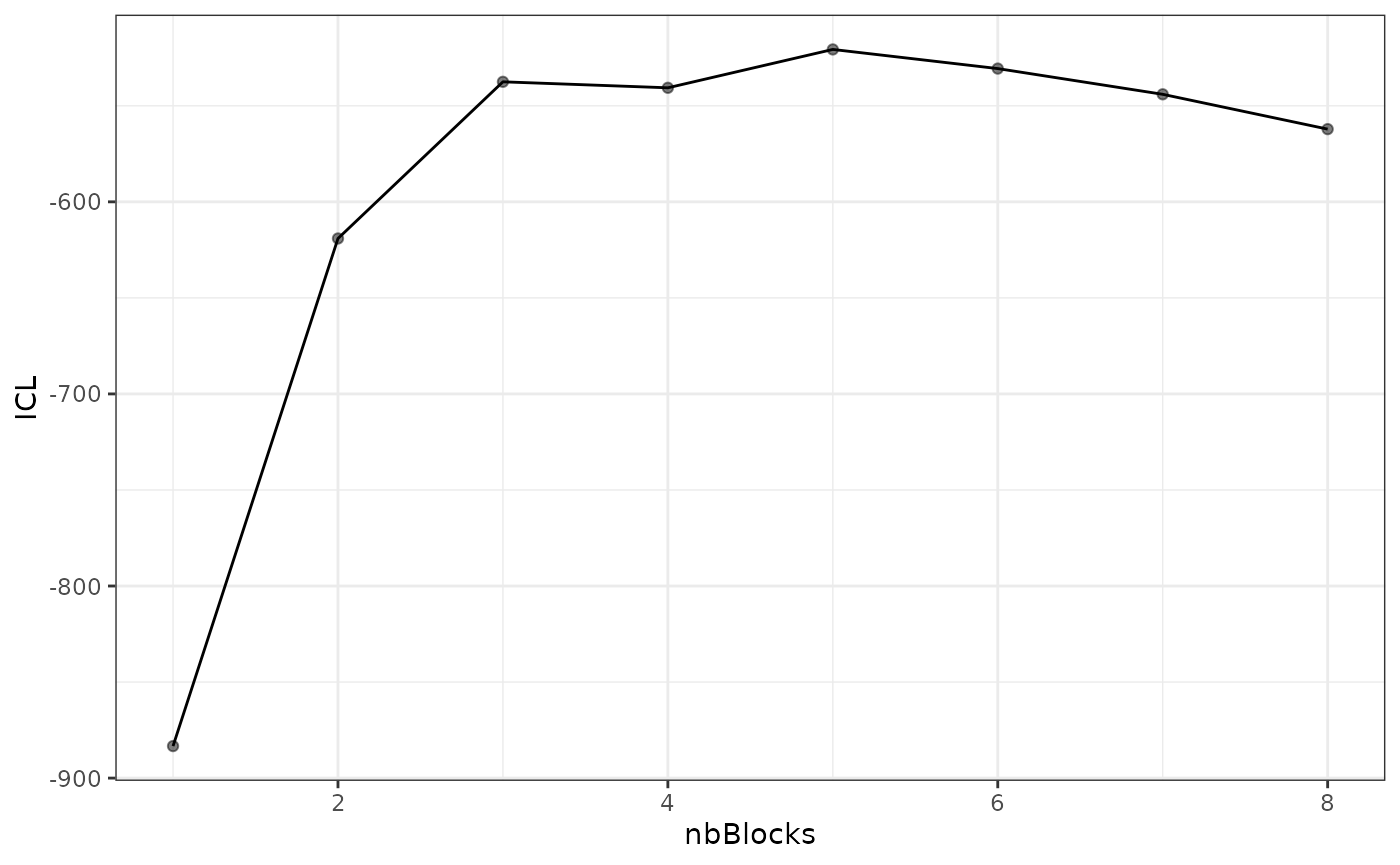

The 4-block model could have been a good choice too, in place of the 5-block model. The user can update the current simpleSBMfit thanks to the the setModel method:

mySimpleSBM$setModel(4)
mySimpleSBM$nbBlocks
#> [1] 4
mySimpleSBM$plot(type = 'expected')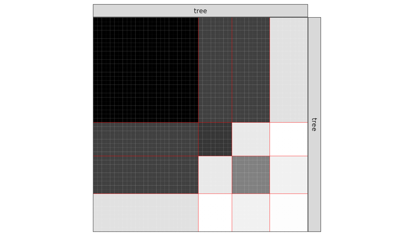

mySimpleSBM$setModel(5)

Analysis of the weighted interaction network

Instead of considering the binary network tree-tree we may consider the weighted network where the link between two trees is the number of fungi they share.

We plot the matrix with function plotMyMatrix:

tree_tree <- fungusTreeNetwork$tree_tree
plotMyMatrix(tree_tree, dimLabels = c('tree'))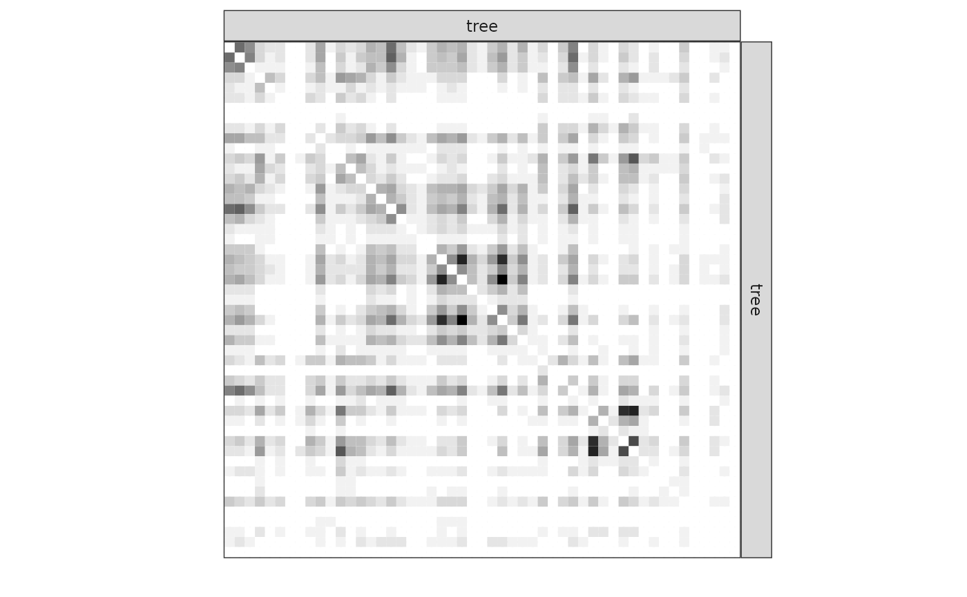

Here again, we look for some latent structure of the network by adjusting a simple SBM with the function estimateSimpleSBM, considering a Poisson distribution on the edges.

mySimpleSBMPoisson <- tree_tree %>% 
  estimateSimpleSBM("poisson", dimLabels = 'tree', estimOptions = list(verbosity = 0, plot = FALSE))

class(mySimpleSBMPoisson)
#> [1] "SimpleSBM_fit" "SimpleSBM"     "SBM"           "R6"
mySimpleSBMPoisson
#> Fit of a Simple Stochastic Block Model -- poisson variant
#> =====================================================================
#> Dimension = ( 51 ) - ( 6 ) blocks and no covariate(s).
#> =====================================================================
#> * Useful fields 
#>   $nbNodes, $modelName, $dimLabels, $nbBlocks, $nbCovariates, $nbDyads
#>   $blockProp, $connectParam, $covarParam, $covarList, $covarEffect 
#>   $expectation, $indMemberships, $memberships 
#> * R6 and S3 methods 
#>   $rNetwork, $rMemberships, $rEdges, plot, print, coef 
#> * Additional fields
#>   $probMemberships, $loglik, $ICL, $storedModels, 
#> * Additional methods 
#>   predict, fitted, $setModel, $reorder

For instance,

mySimpleSBMPoisson$nbBlocks
#> [1] 6
mySimpleSBMPoisson$nbNodes
#> tree 
#>   51
mySimpleSBMPoisson$nbCovariates
#> [1] 0

We now plot the matrix reordered according to the memberships estimated in the SBM:

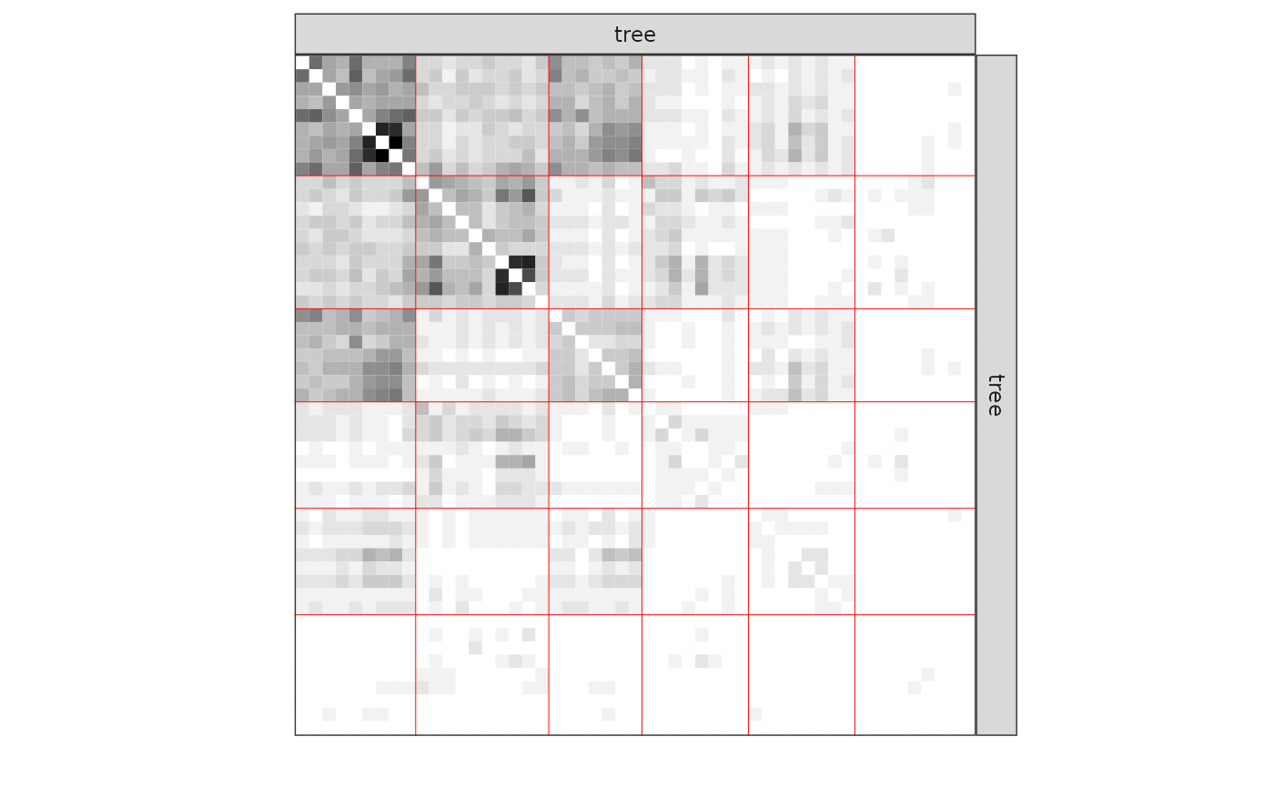
plot(mySimpleSBMPoisson, type = "data", dimLabels =c('tree'))

One can also plot the expected network which, in case of the Poisson model, corresponds to the expectation of connection between any pair of nodes in the network.

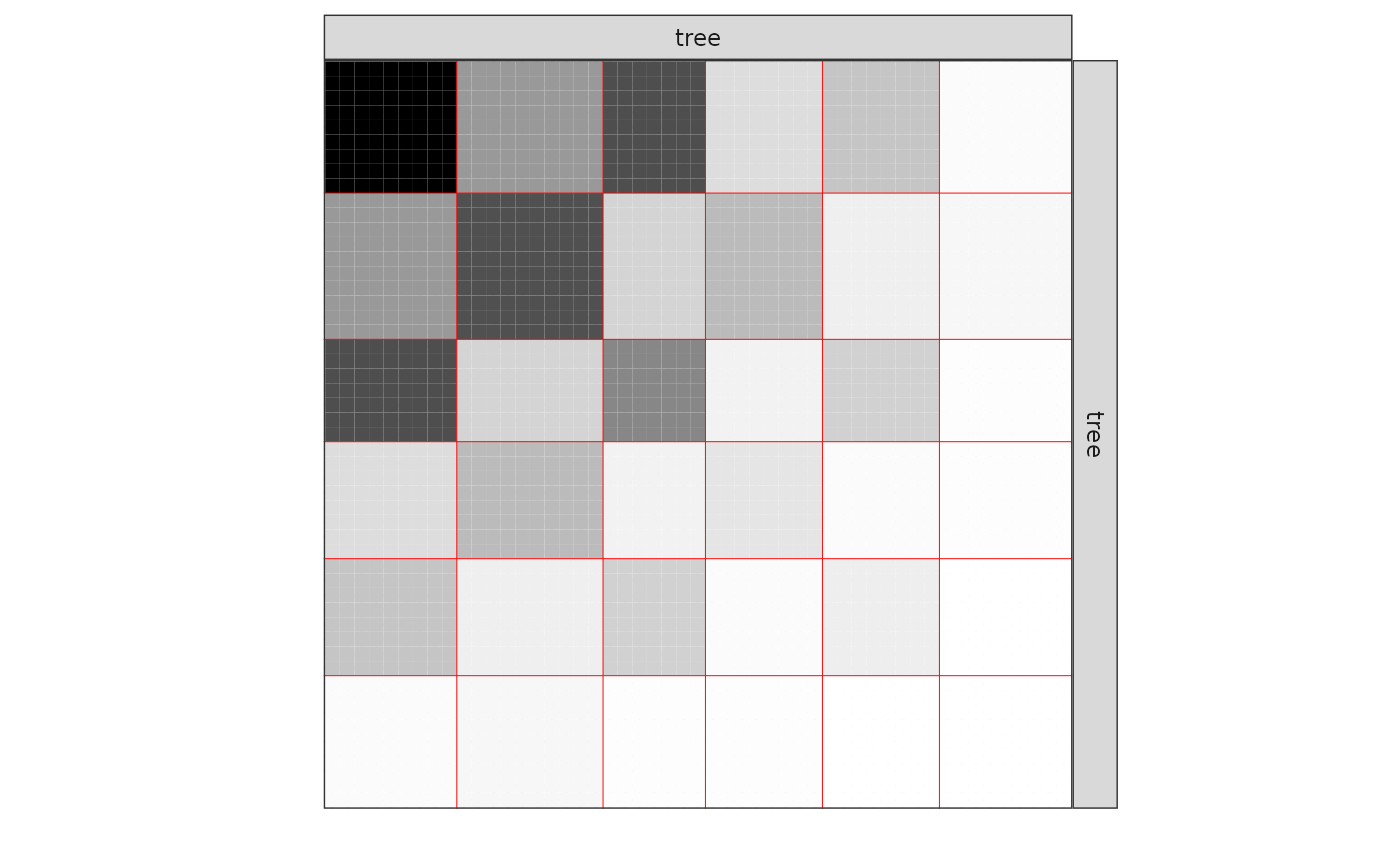
plot(mySimpleSBMPoisson, type = "expected", dimLabels = c('tree'))

plot(mySimpleSBMPoisson, type = "meso")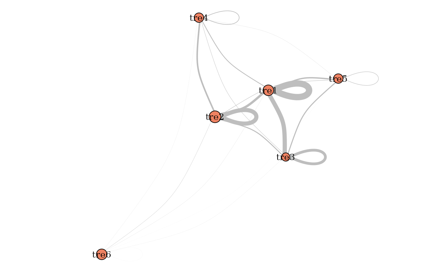

The same manipulations can be made on the models as before.

coef(mySimpleSBMPoisson, 'block')
#> [1] 0.1763561 0.1957351 0.1375982 0.1569772 0.1569772 0.1763561
coef(mySimpleSBMPoisson, 'connectivity')
#> $mean
#>           [,1]      [,2]       [,3]       [,4]       [,5]       [,6]
#> [1,] 9.0286270 3.2910355 6.04727443 1.06850270 1.85464212 0.11062572
#> [2,] 3.2910355 5.9646020 1.33637565 2.17610068 0.49999123 0.26547703
#> [3,] 6.0472744 1.3363757 3.94065914 0.40263458 1.46245649 0.07080814
#> [4,] 1.0685027 2.1761007 0.40263458 0.82166374 0.14089332 0.07793391
#> [5,] 1.8546421 0.4999912 1.46245649 0.14089332 0.54121406 0.02263218
#> [6,] 0.1106257 0.2654770 0.07080814 0.07793391 0.02263218 0.02940543

Introduction of covariates

We have on each pair of trees 3 covariates, namely the genetic distance, the taxonomic distance and the geographic distance. Each covariate has to be introduced as a matrix: $X^k_{ij}$ corresponds to the value of the $k$ -th covariate describing the couple $(i,j)$ .

mySimpleSBMCov<- 
  tree_tree %>% 
  estimateSimpleSBM(
    model = 'poisson', 
    directed = FALSE, 
    dimLabels = 'tree',
    covariates  = fungusTreeNetwork$covar_tree, 
    estimOptions = list(verbosity = 0, plot = FALSE, nbCores = 2)
  )

We select the best number of clusters (with respect to the ICL criteria)

mySimpleSBMCov$nbBlocks
#> [1] 4

We can now extract the parameters of interest, namely ( $\lambda$ , $\pi$ ) and the clustering of the nodes.

mySimpleSBMCov$connectParam
#> $mean
#>           [,1]       [,2]      [,3]      [,4]
#> [1,] 28.203992 14.8912245 5.9616968 1.2393019
#> [2,] 14.891225  9.5630078 3.7924302 0.4103065
#> [3,]  5.961697  3.7924302 1.6186169 0.3842198
#> [4,]  1.239302  0.4103065 0.3842198 0.1893406
mySimpleSBMCov$blockProp
#> [1] 0.3715916 0.2159544 0.2354118 0.1770423
mySimpleSBMCov$memberships
#>  [1] 1 1 2 1 2 2 4 4 2 1 3 1 1 1 1 2 1 2 3 3 2 1 2 1 3 3 2 1 3 2 3 1 4 1 1 3 1 3
#> [39] 4 1 1 3 2 4 4 1 4 4 3 3 4
mySimpleSBMCov$covarParam
#>            [,1]
#> [1,]  0.1974181
#> [2,] -2.0552202
#> [3,] -0.3583405

coef(mySimpleSBMCov, 'covariates')
#>            [,1]
#> [1,]  0.1974181
#> [2,] -2.0552202
#> [3,] -0.3583405

S3 methods are also available for fit and prediction (results hidden here)

#fitted(mySimpleSBMCov)
#predict(mySimpleSBMCov)
#predict(mySimpleSBMCov, fungusTreeNetwork$covar_tree)

Analysis of the tree/fungi data

We now analyze the bipartite tree/fungi interactions. The incidence matrix can be plotted with the function

plotMyMatrix(fungusTreeNetwork$fungus_tree, dimLabels = c(row = 'fungis', col= 'tree'))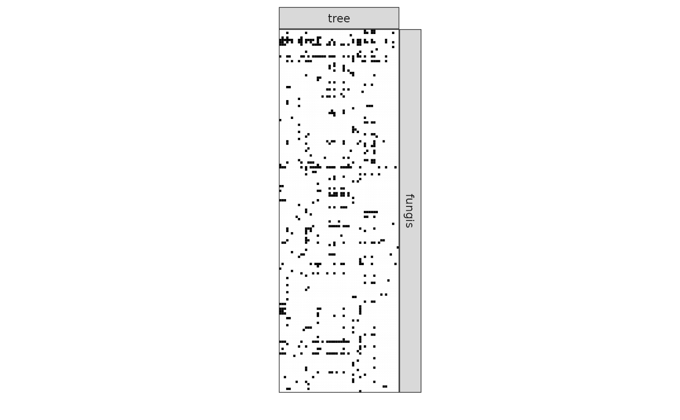

myBipartiteSBM <- 
  fungusTreeNetwork$fungus_tree %>% 
  estimateBipartiteSBM(model = 'bernoulli', dimLabels = c('fungis', 'tree'),estimOptions = list(verbosity = 0, plot = FALSE))

myBipartiteSBM$nbNodes
#> fungis   tree 
#>    154     51
myBipartiteSBM$nbBlocks
#> fungis   tree 
#>      4      4
myBipartiteSBM$connectParam
#> $mean
#>            [,1]        [,2]        [,3]        [,4]
#> [1,] 0.96813478 0.077538579 0.840370657 0.067563355
#> [2,] 0.52055882 0.584398216 0.230893917 0.107930384
#> [3,] 0.32450427 0.003624764 0.098526840 0.005780612
#> [4,] 0.01834547 0.154334411 0.001330278 0.019219920
coef(myBipartiteSBM, 'block')
#> $row
#> [1] 0.02655516 0.05570334 0.31666508 0.60107642
#> 
#> $col
#> [1] 0.1050494 0.1963968 0.2477304 0.4508234
coef(myBipartiteSBM, 'connectivity')
#> $mean
#>            [,1]        [,2]        [,3]        [,4]
#> [1,] 0.96813478 0.077538579 0.840370657 0.067563355
#> [2,] 0.52055882 0.584398216 0.230893917 0.107930384
#> [3,] 0.32450427 0.003624764 0.098526840 0.005780612
#> [4,] 0.01834547 0.154334411 0.001330278 0.019219920

We can now plot the reorganized matrix.

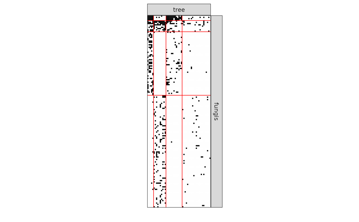
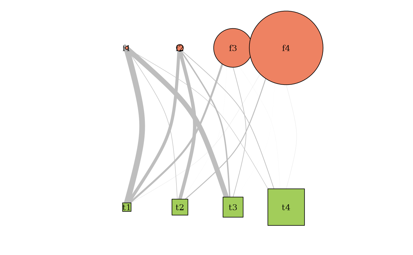
plot(myBipartiteSBM, dimLabels = c('fungis', 'tree'))

plot(myBipartiteSBM, type  = 'meso', 
     dimLabels = list(row = 'fungis', col= 'tree'),
     plotOptions = list(edge.width = 1, vertex.size = c(1,2)))

References

Leger, Jean-Benoist. 2016. “Blockmodels: A r-Package for Estimating in Latent Block Model and Stochastic Block Model, with Various Probability Functions, with or Without Covariates.” arXiv Preprint arXiv:1602.07587.

Vacher, Corinne, Dominique Piou, and Marie-Laure Desprez-Loustau. 2008. “Architecture of an Antagonistic Tree/Fungus Network: The Asymmetric Influence of Past Evolutionary History.” PloS One 3 (3): e1740.

An illustration on antagonistic tree/fungus network

team großBM

2024-09-16