This function performs variational inference of simple Stochastic Block Models, with various model for the distribution of the edges: Bernoulli, Poisson, or Gaussian models.
estimateSimpleSBM(
  netMat,
  model = "bernoulli",
  directed = !isSymmetric(netMat),
  dimLabels = c("node"),
  covariates = list(),
  estimOptions = list()
)
Arguments
- netMat
a matrix describing the network: either an adjacency (square) or incidence matrix with possibly weighted entries.
- model
character describing the model for the relation between nodes (
'bernoulli','poisson','gaussian', ...). Default is'bernoulli'.- directed
logical: is the network directed or not? Only relevant when
typeis'Simple'. Default isTRUEifnetMatis symmetric,FALSEotherwise- dimLabels
an optional label for referring to the nodes
- covariates
a list of matrices with same dimension as mat describing covariates at the edge level. No covariate per Default.
- estimOptions
a list of parameters controlling the inference algorithm and model selection. See details.
Value
a list with the estimated parameters. See details...
Details
The list of parameters estimOptions essentially tunes the optimization process and the variational EM algorithm, with the following parameters
"nbCores integer for number of cores used. Default is 2
"verbosity" integer for verbosity (0, 1). Default is 1
"plot" boolean, should the ICL by dynamically plotted or not. Default is TRUE
"exploreFactor" control the exploration of the number of groups
"exploreMin" explore at least until exploreMin even if the exploration factor rule is achieved. Default 4. See the package blockmodels for details.
"exploreMax" Stop exploration at exploreMax even if the exploration factor rule is not achieved. Default Inf. See the package blockmodels for details.
"nbBlocksRange" minimal and maximal number or blocks explored
"fast" logical: should approximation be used for Bernoulli model with covariates. Default to
TRUE
Examples
### =======================================
### SIMPLE BINARY SBM (Bernoulli model)
## Graph parameters & Sampling
nbNodes <- 60
blockProp <- c(.5, .25, .25) # group proportions
means <- diag(.4, 3) + 0.05 # connectivity matrix: affiliation network
connectParam <- list(mean = means)
mySampler <- sampleSimpleSBM(nbNodes, blockProp, connectParam)
adjacencyMatrix <- mySampler$networkData
## Estimation
mySimpleSBM <-
estimateSimpleSBM(adjacencyMatrix, 'bernoulli', estimOptions = list(plot = FALSE))
#> -> Estimation for 1 groups
#>
-> Computation of eigen decomposition used for initalizations
#>
#> -> Pass 1
#> -> With ascending number of groups
#> -> For 2 groups
#>
-> For 3 groups
#>
-> For 4 groups
#>
-> For 5 groups
#>
-> With descending number of groups
#> -> For 4 groups
#>
-> For 3 groups
#>
-> For 2 groups
#>
-> Pass 2
#> -> With ascending number of groups
#> -> For 2 groups
#> -> For 3 groups
#> -> For 4 groups
#> -> For 5 groups
#> -> With descending number of groups
#> -> For 4 groups
#> -> For 3 groups
#> -> For 2 groups
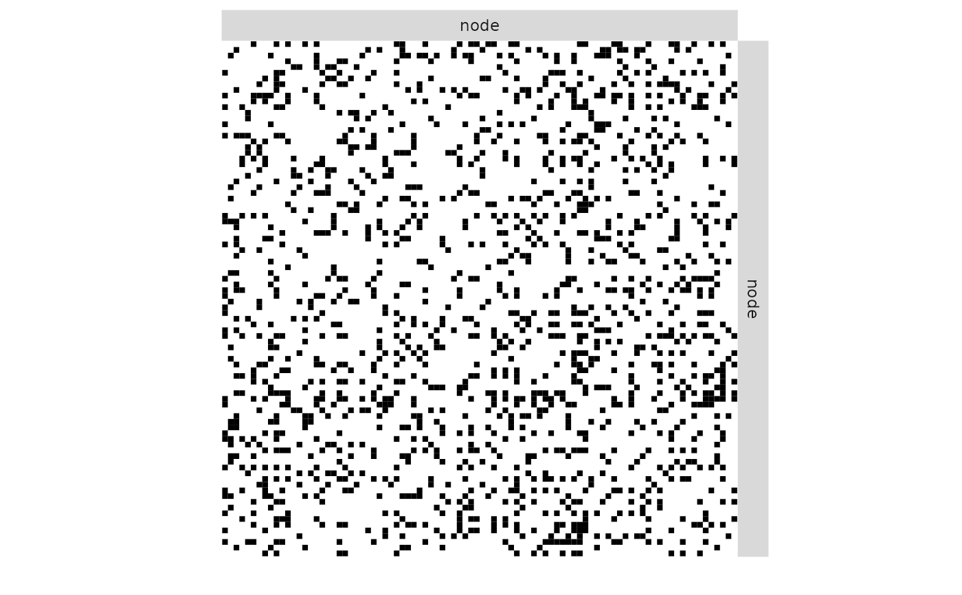
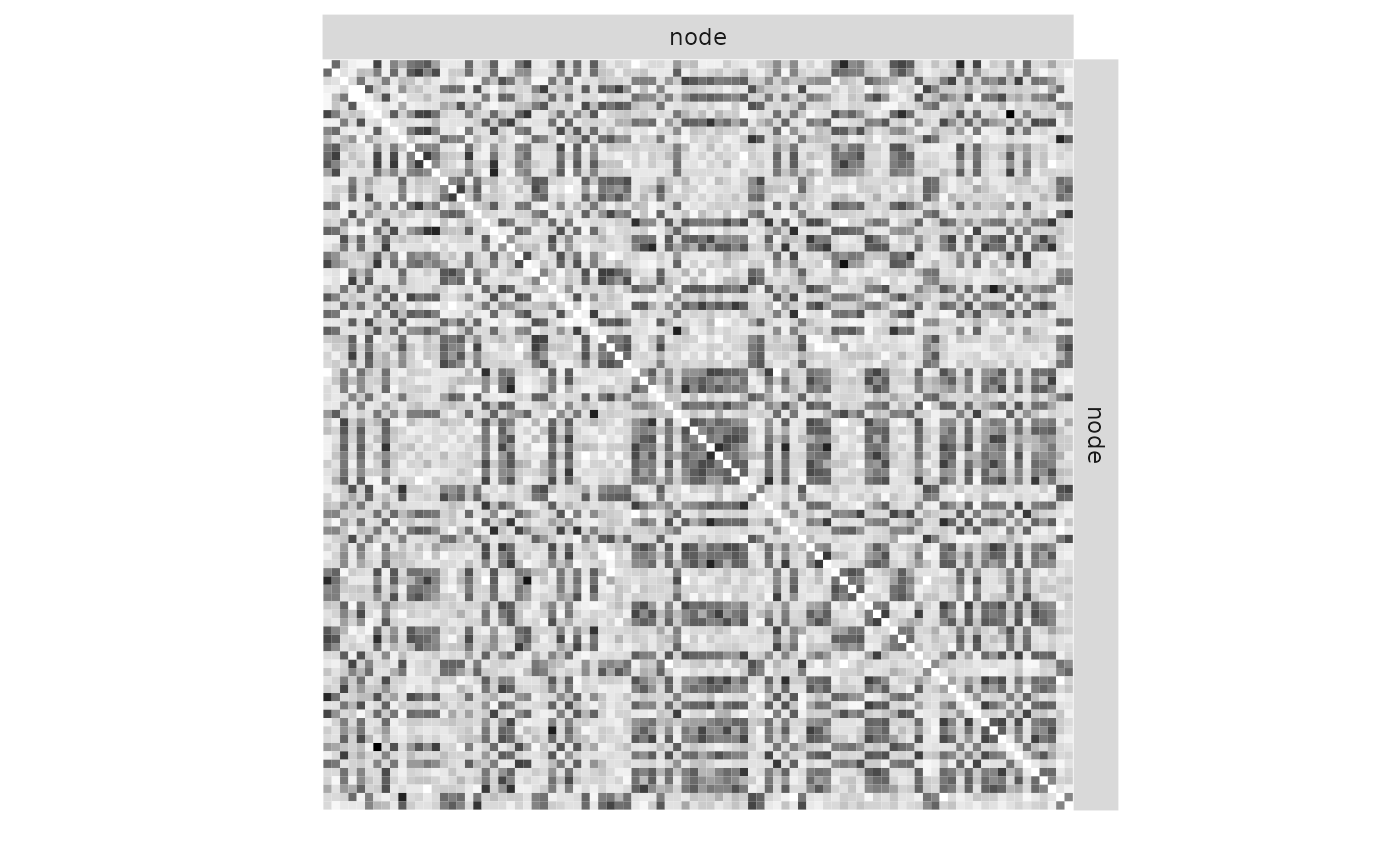
plot(mySimpleSBM, 'data', ordered = FALSE)
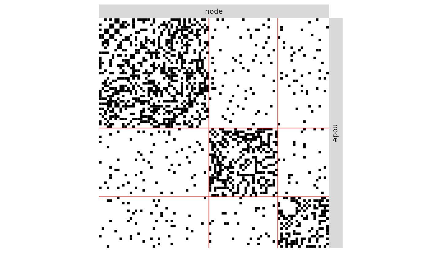
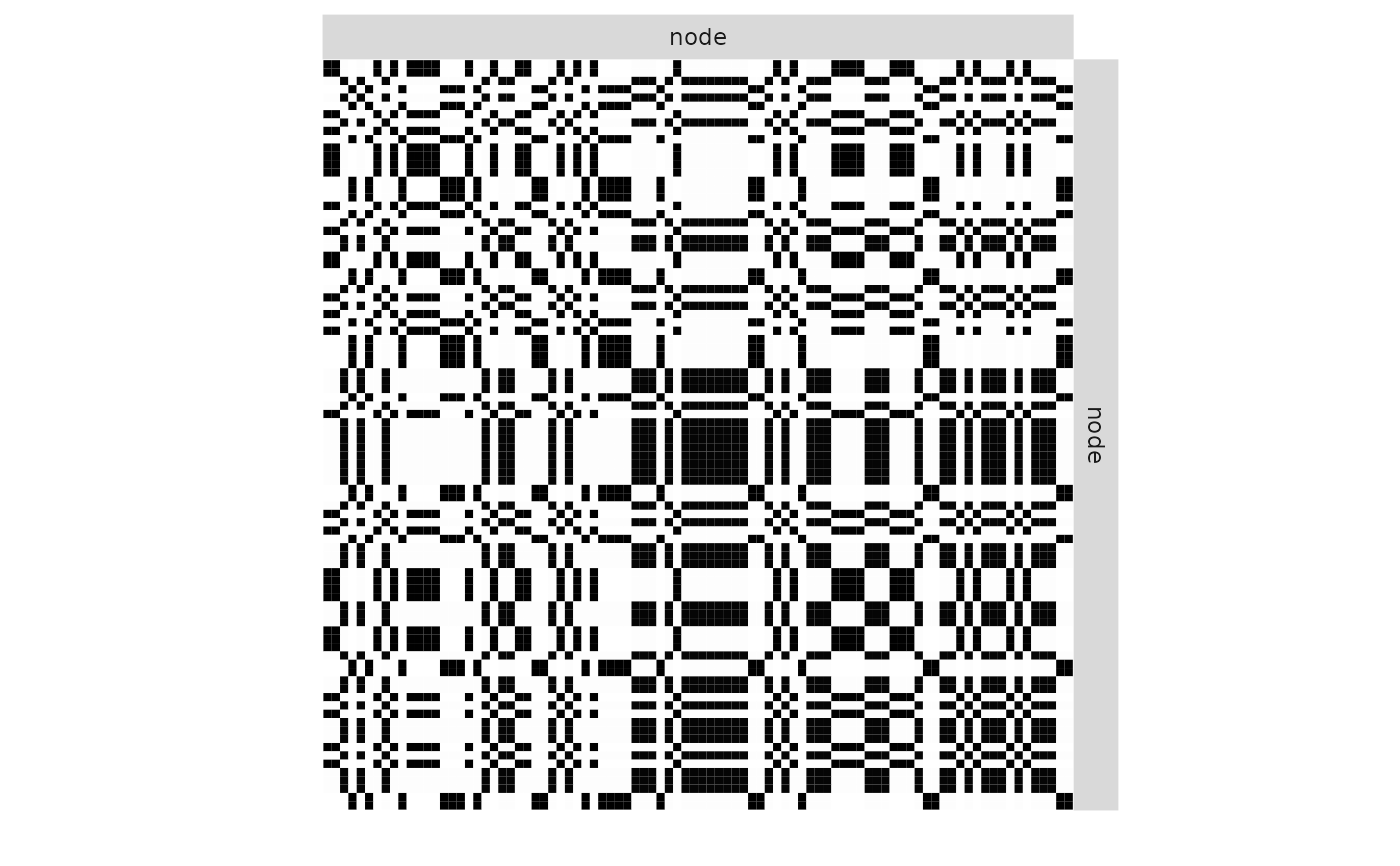
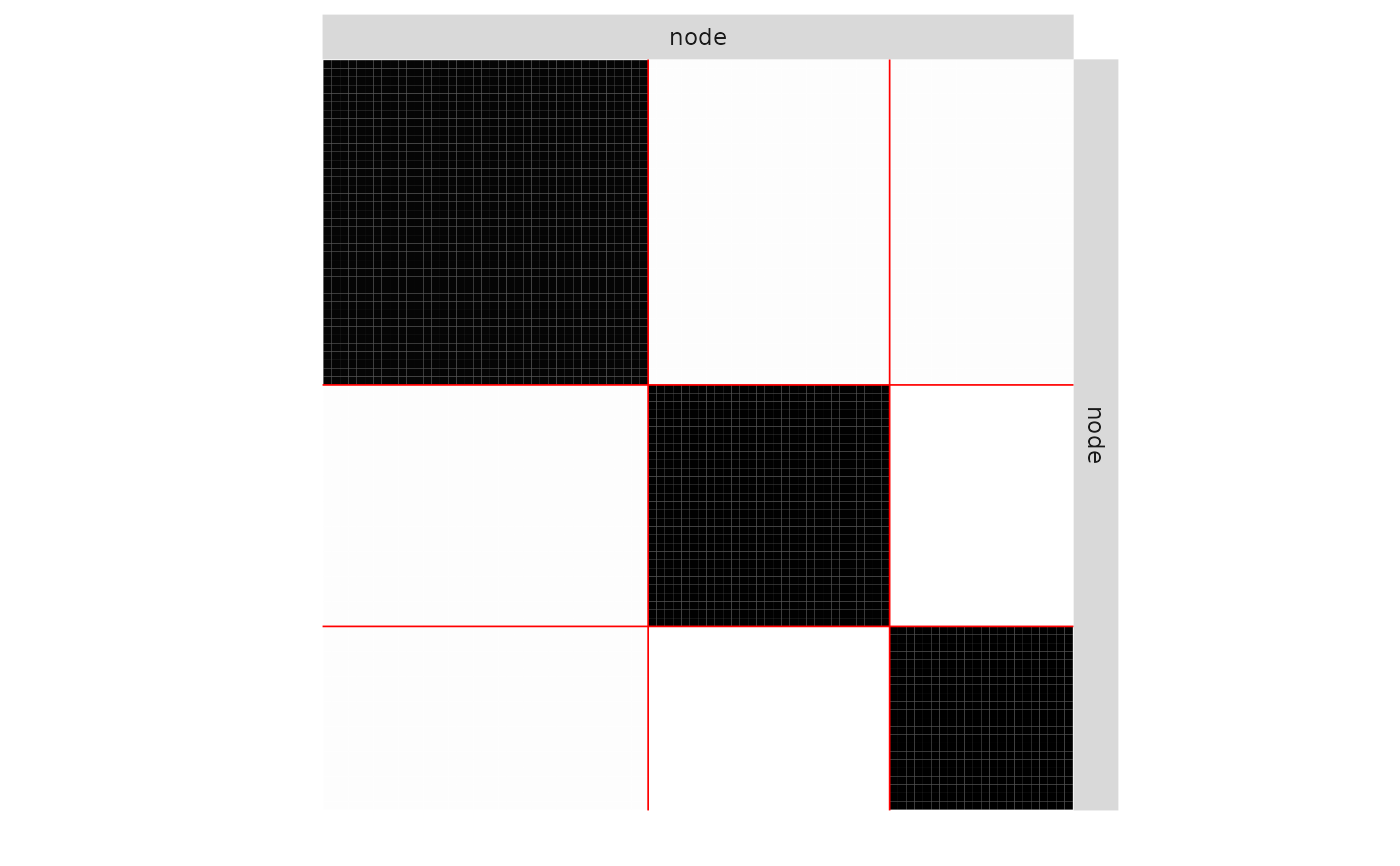
 plot(mySimpleSBM, 'data')
 plot(mySimpleSBM, 'expected', ordered = FALSE)
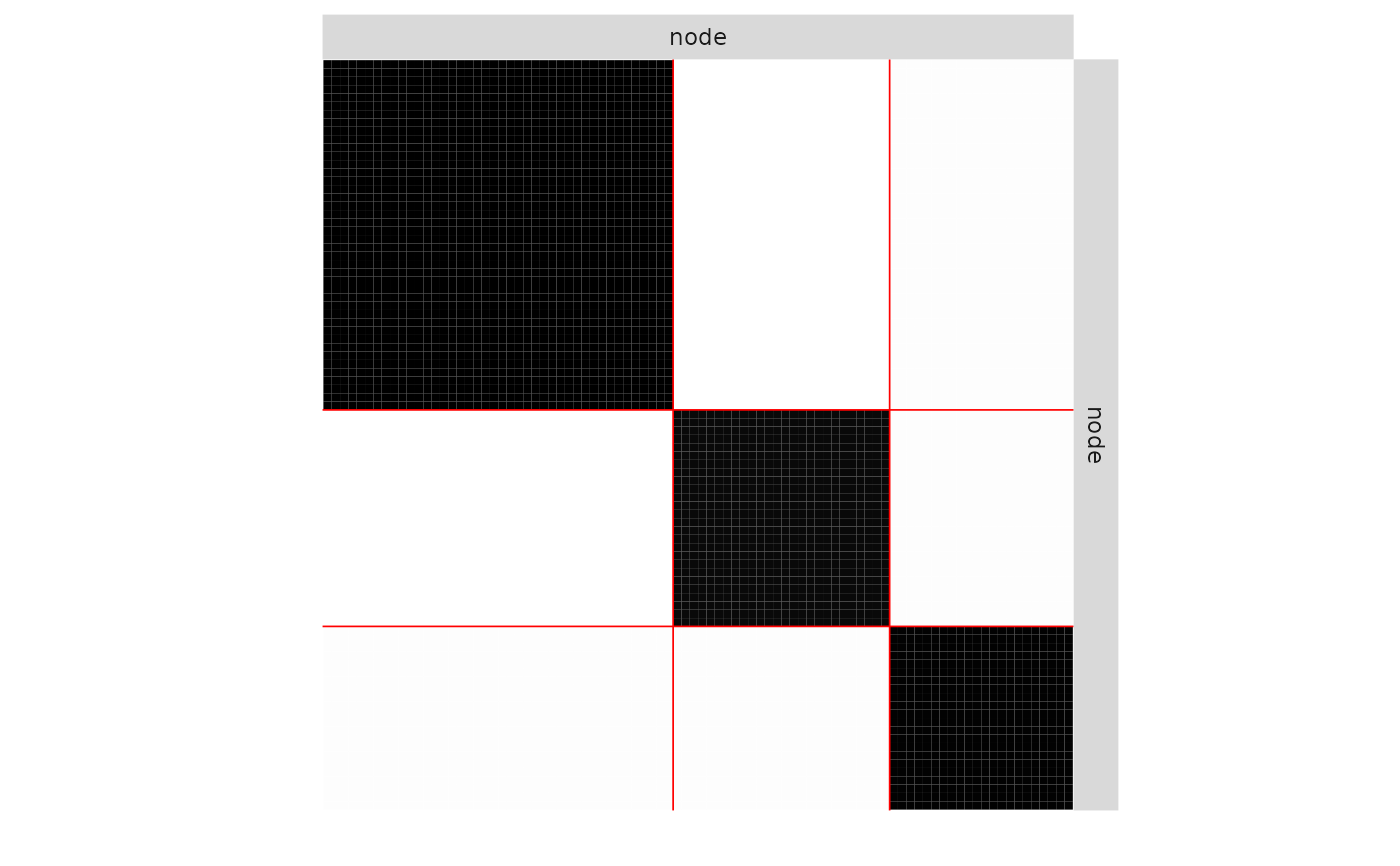
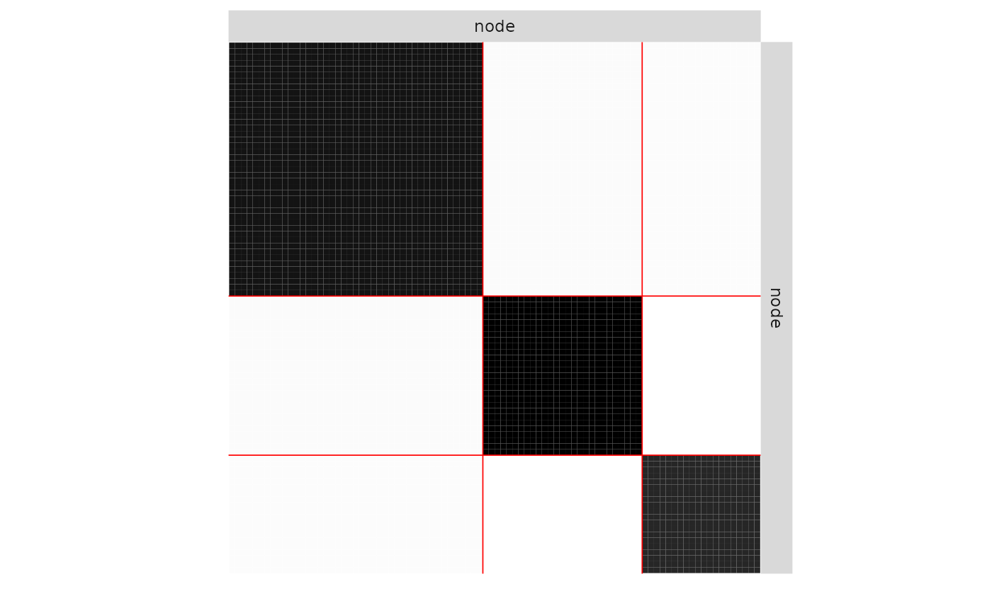
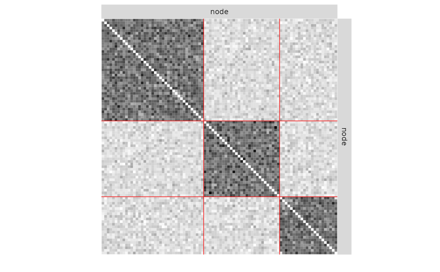
 plot(mySimpleSBM, 'expected')
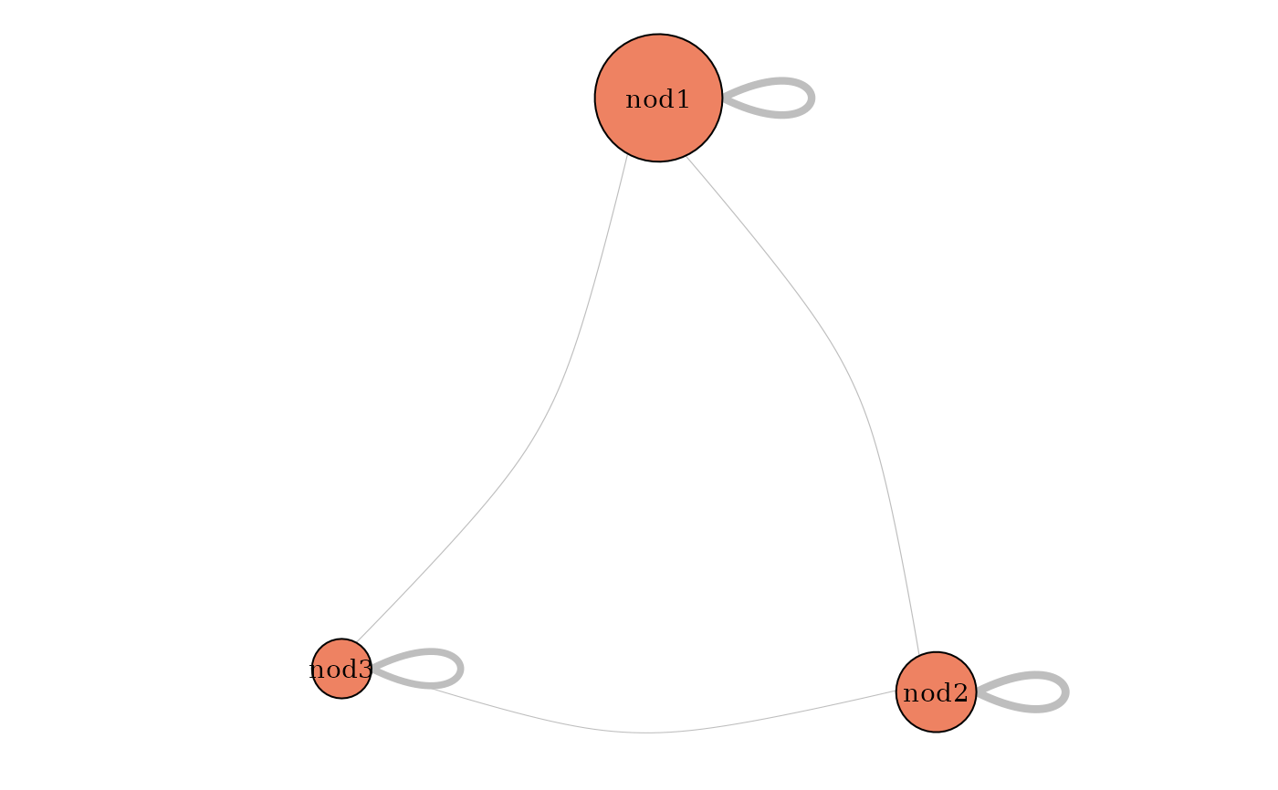
 plot(mySimpleSBM, 'meso')
 ### =======================================
### SIMPLE POISSON SBM
## Graph parameters & Sampling
nbNodes <- 60
blockProp <- c(.5, .25, .25) # group proportions
means <- diag(15., 3) + 5 # connectivity matrix: affiliation network
connectParam <- list(mean = means)
mySampler <- sampleSimpleSBM(nbNodes, blockProp, list(mean = means), model = "poisson")
adjacencyMatrix <- mySampler$networkData
## Estimation
mySimpleSBM <- estimateSimpleSBM(adjacencyMatrix, 'poisson',
estimOptions = list(plot = FALSE))
#> -> Estimation for 1 groups
#>
-> Computation of eigen decomposition used for initalizations
#>
#> -> Pass 1
#> -> With ascending number of groups
#> -> For 2 groups
#>
-> For 3 groups
#>
-> For 4 groups
#>
-> For 5 groups
#>
-> With descending number of groups
#> -> For 4 groups
#>
-> For 3 groups
#>
-> For 2 groups
#>
-> Pass 2
#> -> With ascending number of groups
#> -> For 2 groups
#> -> For 3 groups
#> -> For 4 groups
#> -> For 5 groups
#> -> With descending number of groups
#> -> For 4 groups
#> -> For 3 groups
#> -> For 2 groups
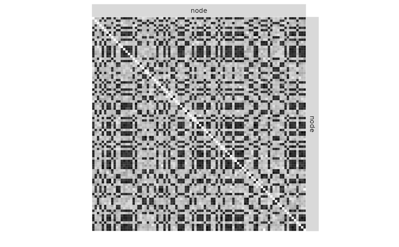
plot(mySimpleSBM, 'data', ordered = FALSE)
### =======================================
### SIMPLE POISSON SBM
## Graph parameters & Sampling
nbNodes <- 60
blockProp <- c(.5, .25, .25) # group proportions
means <- diag(15., 3) + 5 # connectivity matrix: affiliation network
connectParam <- list(mean = means)
mySampler <- sampleSimpleSBM(nbNodes, blockProp, list(mean = means), model = "poisson")
adjacencyMatrix <- mySampler$networkData
## Estimation
mySimpleSBM <- estimateSimpleSBM(adjacencyMatrix, 'poisson',
estimOptions = list(plot = FALSE))
#> -> Estimation for 1 groups
#>
-> Computation of eigen decomposition used for initalizations
#>
#> -> Pass 1
#> -> With ascending number of groups
#> -> For 2 groups
#>
-> For 3 groups
#>
-> For 4 groups
#>
-> For 5 groups
#>
-> With descending number of groups
#> -> For 4 groups
#>
-> For 3 groups
#>
-> For 2 groups
#>
-> Pass 2
#> -> With ascending number of groups
#> -> For 2 groups
#> -> For 3 groups
#> -> For 4 groups
#> -> For 5 groups
#> -> With descending number of groups
#> -> For 4 groups
#> -> For 3 groups
#> -> For 2 groups
plot(mySimpleSBM, 'data', ordered = FALSE)
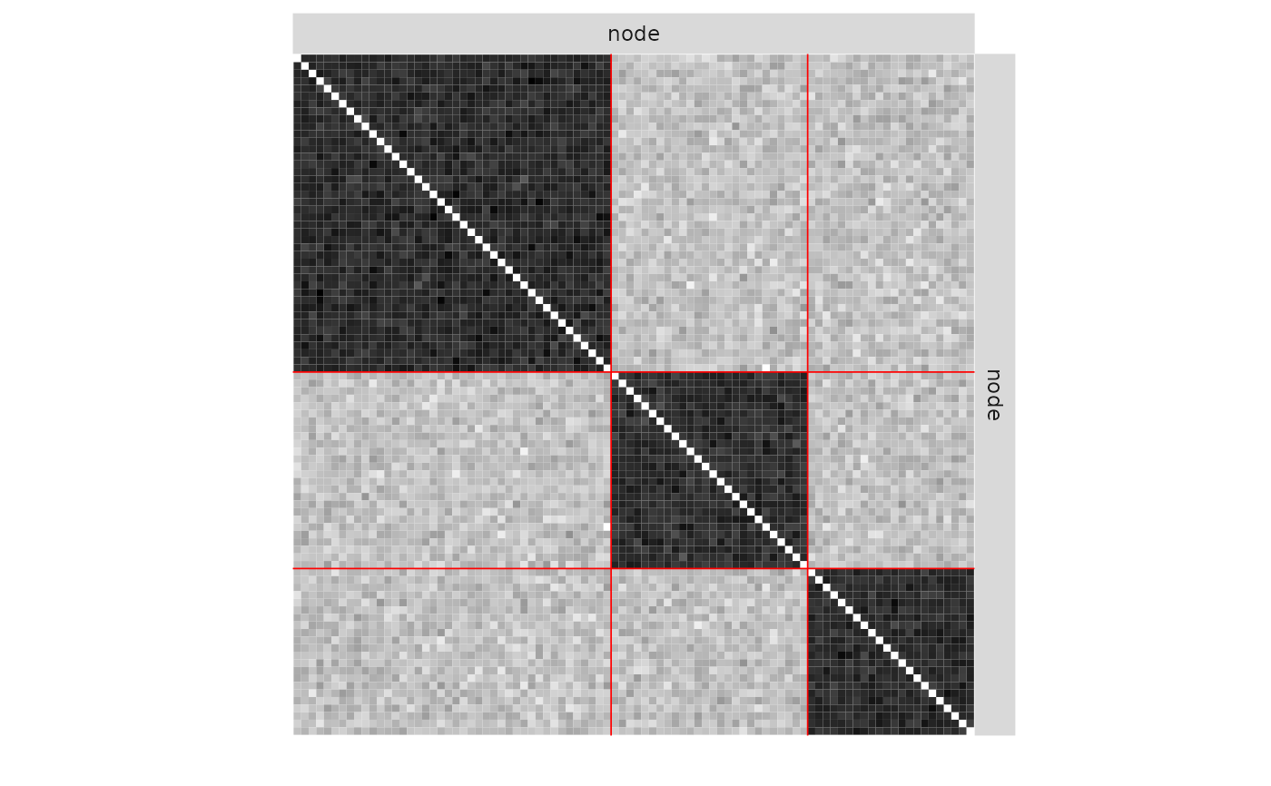
 plot(mySimpleSBM, 'data')
 plot(mySimpleSBM, 'expected', ordered = FALSE)
 plot(mySimpleSBM, 'expected')
 ### =======================================
### SIMPLE GAUSSIAN SBM
## Graph parameters & Sampling
nbNodes <- 60
blockProp <- c(.5, .25, .25) # group proportions
means <- diag(15., 3) + 5 # connectivity matrix: affiliation network
connectParam <- list(mean = means, var = 2)
mySampler <- sampleSimpleSBM(nbNodes, blockProp, connectParam, model = "gaussian")
## Estimation
mySimpleSBM <-
estimateSimpleSBM(mySampler$networkData, 'gaussian', estimOptions = list(plot = FALSE))
#> -> Estimation for 1 groups
#>
-> Computation of eigen decomposition used for initalizations
#>
#> -> Pass 1
#> -> With ascending number of groups
#> -> For 2 groups
#>
-> For 3 groups
#>
-> For 4 groups
#>
-> For 5 groups
#>
-> With descending number of groups
#> -> For 4 groups
#>
-> For 3 groups
#>
-> For 2 groups
#>
-> Pass 2
#> -> With ascending number of groups
#> -> For 2 groups
#> -> For 3 groups
#> -> For 4 groups
#> -> For 5 groups
#> -> With descending number of groups
#> -> For 4 groups
#> -> For 3 groups
#> -> For 2 groups
plot(mySimpleSBM, 'data', ordered = FALSE)
### =======================================
### SIMPLE GAUSSIAN SBM
## Graph parameters & Sampling
nbNodes <- 60
blockProp <- c(.5, .25, .25) # group proportions
means <- diag(15., 3) + 5 # connectivity matrix: affiliation network
connectParam <- list(mean = means, var = 2)
mySampler <- sampleSimpleSBM(nbNodes, blockProp, connectParam, model = "gaussian")
## Estimation
mySimpleSBM <-
estimateSimpleSBM(mySampler$networkData, 'gaussian', estimOptions = list(plot = FALSE))
#> -> Estimation for 1 groups
#>
-> Computation of eigen decomposition used for initalizations
#>
#> -> Pass 1
#> -> With ascending number of groups
#> -> For 2 groups
#>
-> For 3 groups
#>
-> For 4 groups
#>
-> For 5 groups
#>
-> With descending number of groups
#> -> For 4 groups
#>
-> For 3 groups
#>
-> For 2 groups
#>
-> Pass 2
#> -> With ascending number of groups
#> -> For 2 groups
#> -> For 3 groups
#> -> For 4 groups
#> -> For 5 groups
#> -> With descending number of groups
#> -> For 4 groups
#> -> For 3 groups
#> -> For 2 groups
plot(mySimpleSBM, 'data', ordered = FALSE)
 plot(mySimpleSBM, 'data')
 plot(mySimpleSBM, 'expected', ordered = FALSE)
 plot(mySimpleSBM, 'expected')