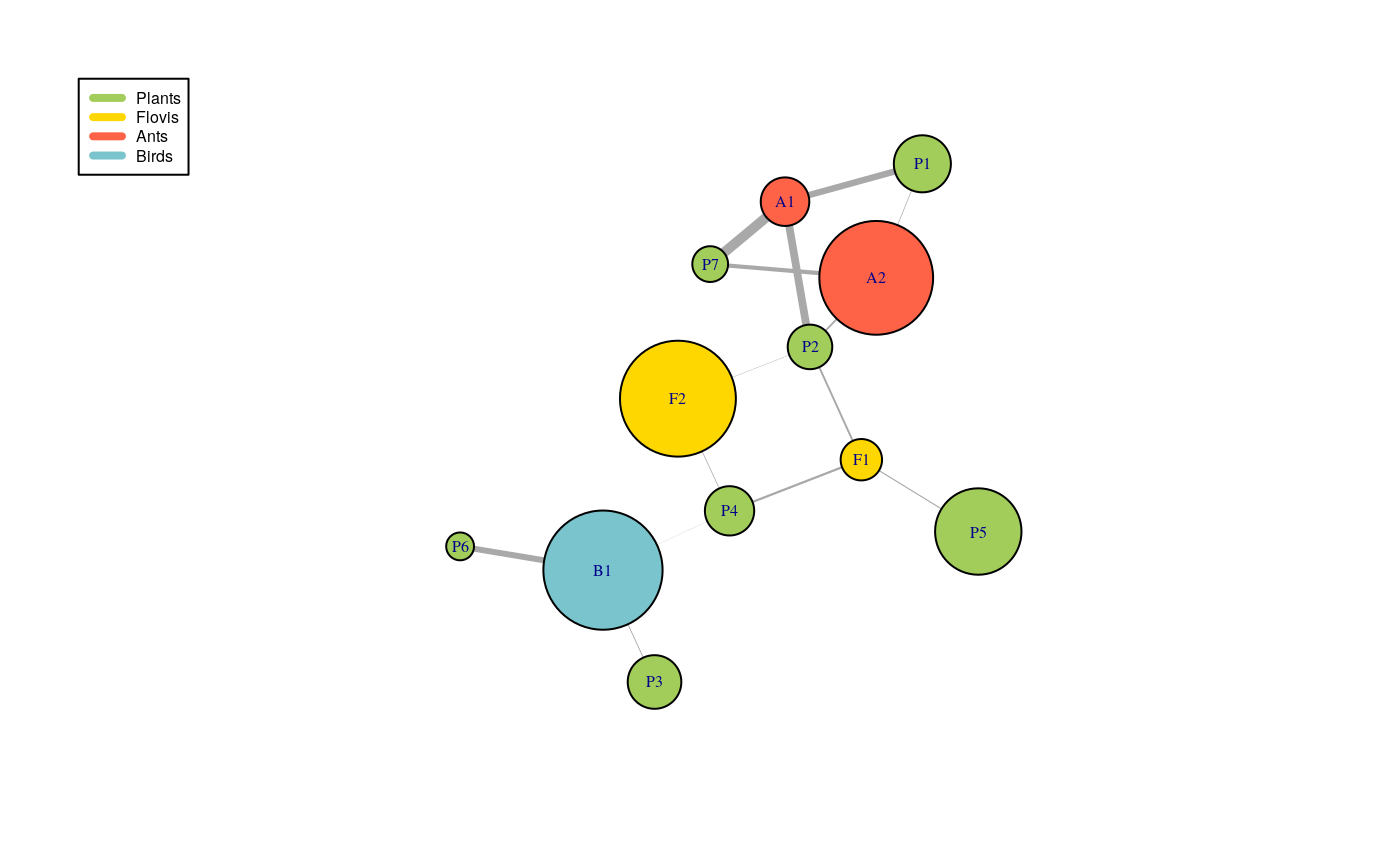
Analysis of a mutualistic multipartite ecological network with GREMLINS

Sophie Donnet, Pierre Barbillon

2020-11-27

The dataset

We apply our methodology to an ecological mutualistic multipartite network.
The dataset –compiled and conducted by Dáttilo et al. (2016) at Centro de Investigaciones Costeras La Mancha (CICOLMA), located on the central coast of the Gulf of Mexico, Veracruz, Mexico– involves three general types of plant-animal mutualistic interaction: pollination, seed dispersal by frugivorous birds, and protective mutualisms between ants and plants with extrafloral nectaries.

The dataset –which is one of the largest compiled so far with respect to species richness, number of interactions and sampling effort– includes 4 functional groups, namely plants, pollinator species (refered as floral visitors), ant species and frugivorous bird species. Three binary bipartite networks have been collected representing interactions between 1/ plants and florals visitor, 2/ plants and ants, and 3/ plants and seed dispersal birds, resulting into three bipartite networks.

The FG are of respective sizes: \(n_1 = 141\) plant species, \(n_2 = 173\) pollinator species (refered as ), \(n_3 = 46\) frugivorous bird species and \(n_4 = 30\) ant species.

The 3 networks contain \(753\) observed interactions of which \(55\%\) are plant-pollinator interactions, \(17\%\) are plant-birds interactions and \(28\%\) are plant-ant interactions.

library(GREMLINS)
data(MPEcoNetwork, package = "GREMLINS")
ls()
#> [1] "MPEcoNetwork"
names(MPEcoNetwork)
#> [1] "Inc_plant_ant"    "Inc_plant_bird"   "Inc_plant_flovis"

As required by GREMLINS, our the global network has to be encoded in separate matrices for each network (in our case the \(3\) incidence matrices) So, here, our 3 networks are provided in 3 incidence matrices, the plants being in rows. Note that the order of the individuals within the functional groups must be the same in all the matrices.

Formatting the data

We format the data to be able to use our R package GREMLINS i.e. we transform the matrices into an list containing the matrix, its type : inc for incidence matrix, adj for adjacency symetric, and diradj for non symetric (oriented) adjacency matrix, the name of functional group in row and the name of functional group in column. The three matrices are gathered in a list.

To do so, we use de the function defineNetwork.

PlantFlovis = defineNetwork(MPEcoNetwork$Inc_plant_flovis,"inc","Plants","Flovis")
PlantAnt = defineNetwork(MPEcoNetwork$Inc_plant_ant,"inc","Plants","Ants")
PlantBird = defineNetwork(MPEcoNetwork$Inc_plant_bird,"inc","Plants","Birds")
list_net <- list(PlantFlovis,PlantAnt,PlantBird)
names(PlantFlovis)
#> [1] "mat"       "typeInter" "rowFG"     "colFG"

If one wants to keep a track of the names of the species, they should be used as rownames and colnames in the matrices.

PlantFlovis$mat[1:2,1:2]
#>                    Apis_melifera Lasioglossum_sp1
#> Acacia_cornigera               0                1
#> Acacia_macracantha             0                0

Inference

The model selection and the estimation are performed with the function multipartiteBM.

RES_MBM = multipartiteBM(
    list_Net =list(PlantFlovis, PlantAnt, PlantBird),
    namesFG = c('Plants','Flovis','Ants','Birds'),
    v_distrib  = c('bernoulli','bernoulli','bernoulli'),
    initBM = TRUE,save = TRUE)

RES_MBM contains the estimated parameters of the models we run through during the search of the better numbers of blocks. If one sets save = FALSE in the multipartiteBM function then we only save the best model.

RES_MBM constains de dataset and the results.

names(RES_MBM)
#> [1] "fittedModel" "list_Net"

The better model has the following numbers of blocks

RES_MBM$fittedModel[[1]]$paramEstim$v_K
#> Plants Flovis   Ants  Birds 
#>      7      2      2      1

To see the parameters estimated for the better model we use the following command RES_MBM$fittedModel[[1]]$paramEstim$***

RES_MBM$fittedModel[[1]]$paramEstim$list_pi$Plants
#> [1] 0.16063183 0.07840873 0.13507513 0.10614897 0.46752510 0.01418720 0.03802305
RES_MBM$fittedModel[[1]]$paramEstim$list_theta$PlantsFlovis
#>              [,1]         [,2]
#> [1,] 4.173707e-03 8.566580e-08
#> [2,] 1.651832e-01 3.427940e-02
#> [3,] 8.826487e-07 3.317267e-04
#> [4,] 1.917898e-01 6.378749e-02
#> [5,] 9.573240e-02 7.490241e-03
#> [6,] 2.464664e-15 4.440892e-16
#> [7,] 1.001131e-15 4.440892e-16

The clustering supplied by the better model are in RES_MBM$fittedModel[[1]]$paramEstim$Z$***.

table(RES_MBM$fittedModel[[1]]$paramEstim$Z$Plants)
#> 
#>  1  2  3  4  5  6  7 
#> 23 11 20 15 65  2  5
table(RES_MBM$fittedModel[[1]]$paramEstim$Z$Ants)
#> 
#>  1  2 
#>  3 27

Plots

par(cex=.5)
plotMBM(RES_MBM,mycol= c("darkolivegreen3", "gold", "tomato","cadetblue3"))

References

Dáttilo, Wesley, Nubia Lara-Rodrı́guez, Pedro Jordano, Paulo R. Guimarães, John N. Thompson, Robert J. Marquis, Lucas P. Medeiros, Raul Ortiz-Pulido, Maria A. Marcos-Garcı́a, and Victor Rico-Gray. 2016. “Unravelling Darwin’s Entangled Bank: Architecture and Robustness of Mutualistic Networks with Multiple Interaction Types.” Proceedings of the Royal Society of London B: Biological Sciences 283 (1843).